Dr. KC Bierlich, Postdoctoral Scholar, OSU Department of Fisheries, Wildlife, & Conservation Sciences, Geospatial Ecology of Marine Megafauna Lab
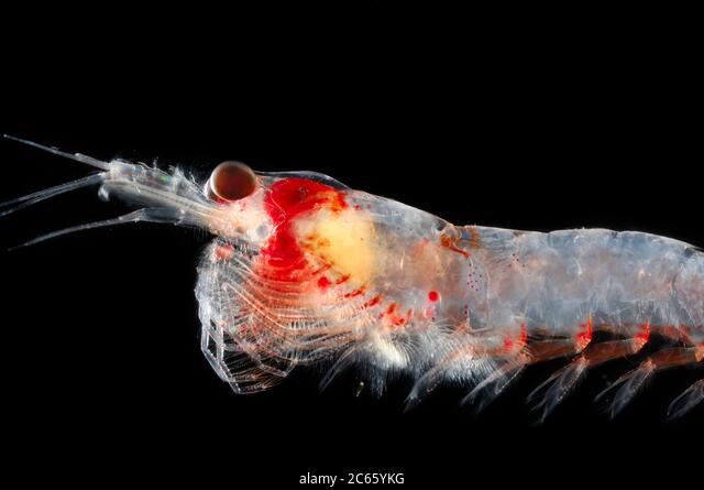
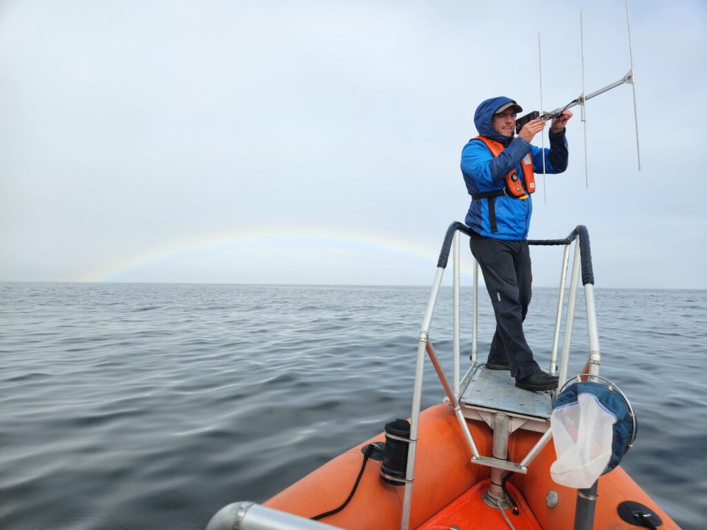
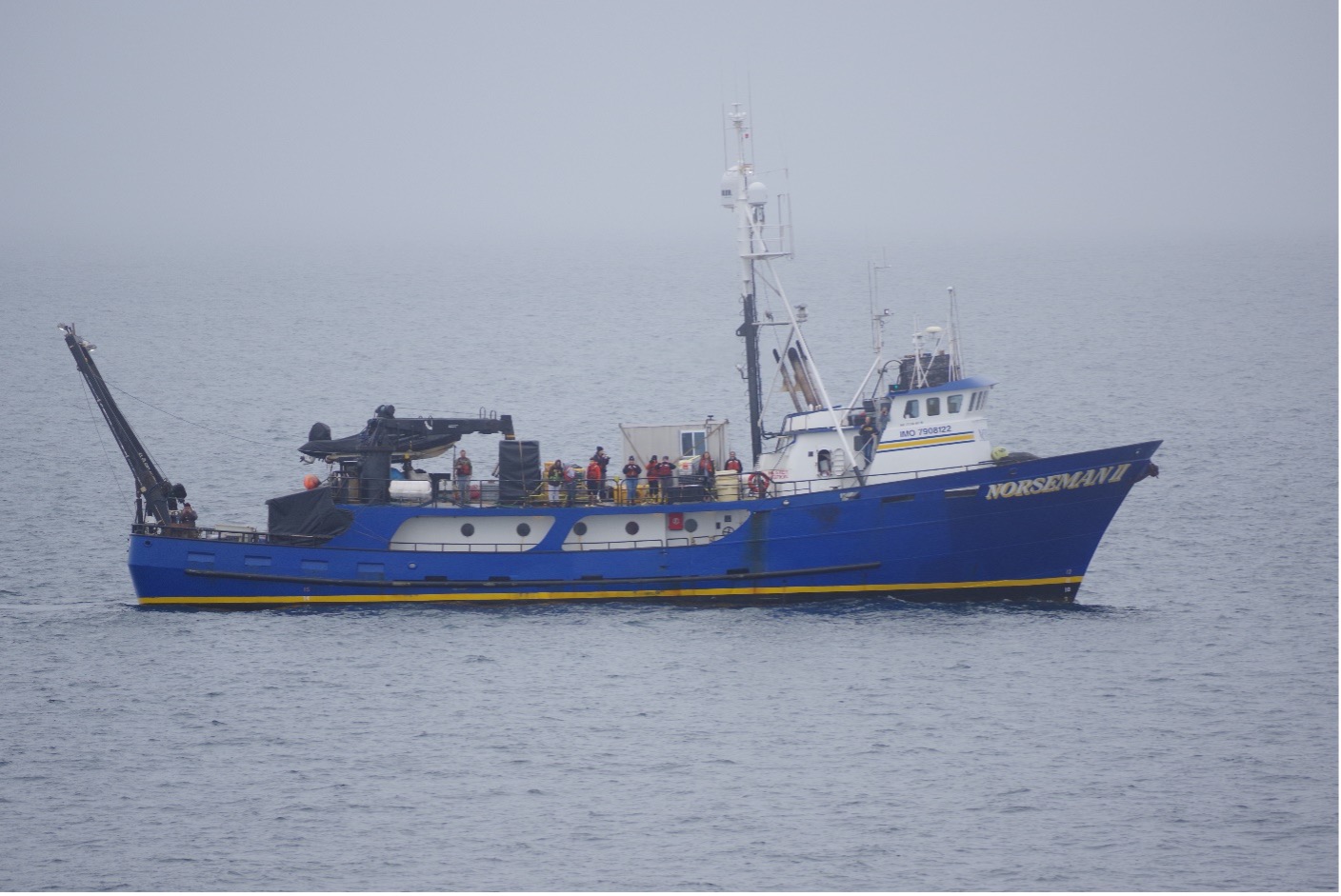
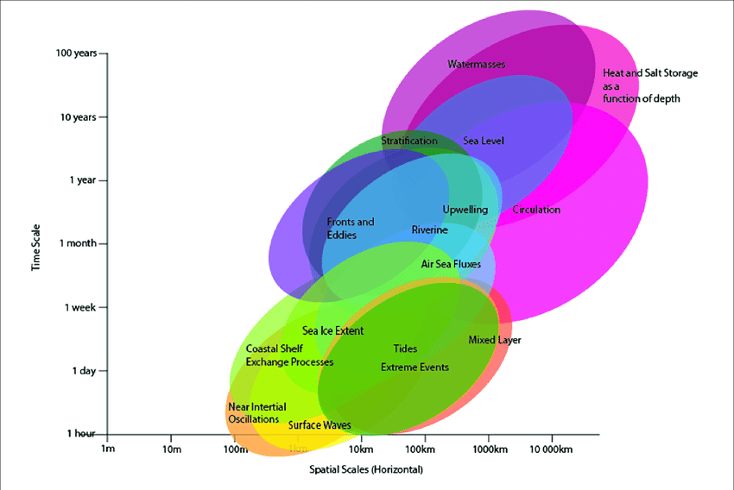
The SAPPHIRE Project is in full swing, as we spend our days aboard the R/V Star Keys searching for krill and blue whales (Figure 1) in the South Taranaki Bight (STB) region of Aotearoa New Zealand. We are investigating how changing ocean conditions impact krill availability and quality, and how this in turn impacts blue whale behavior, health, and reproduction. Understanding the link between changing environmental conditions on prey species and predators is key to understanding the larger implications of climate change on ocean food webs and each populations’ resiliency.

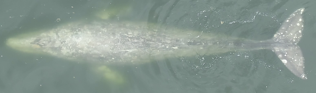
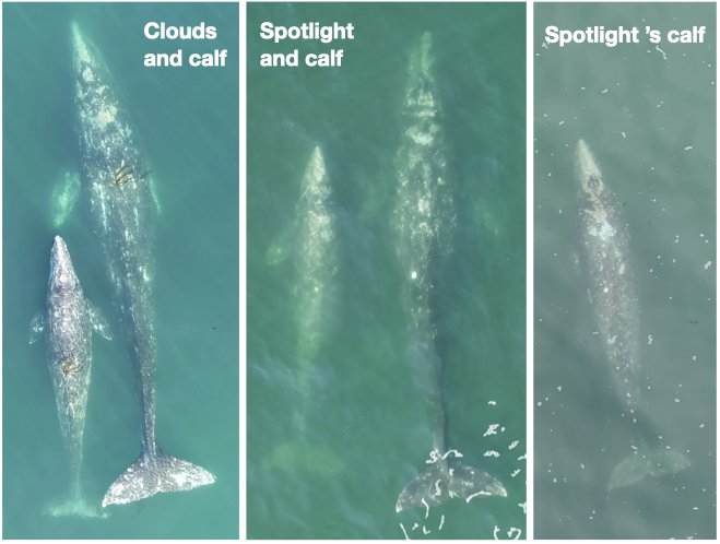
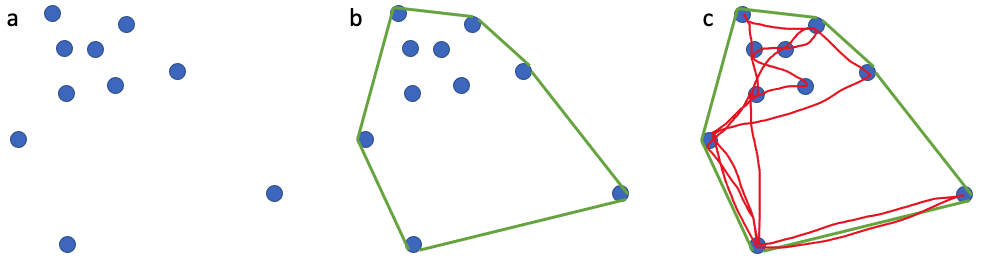
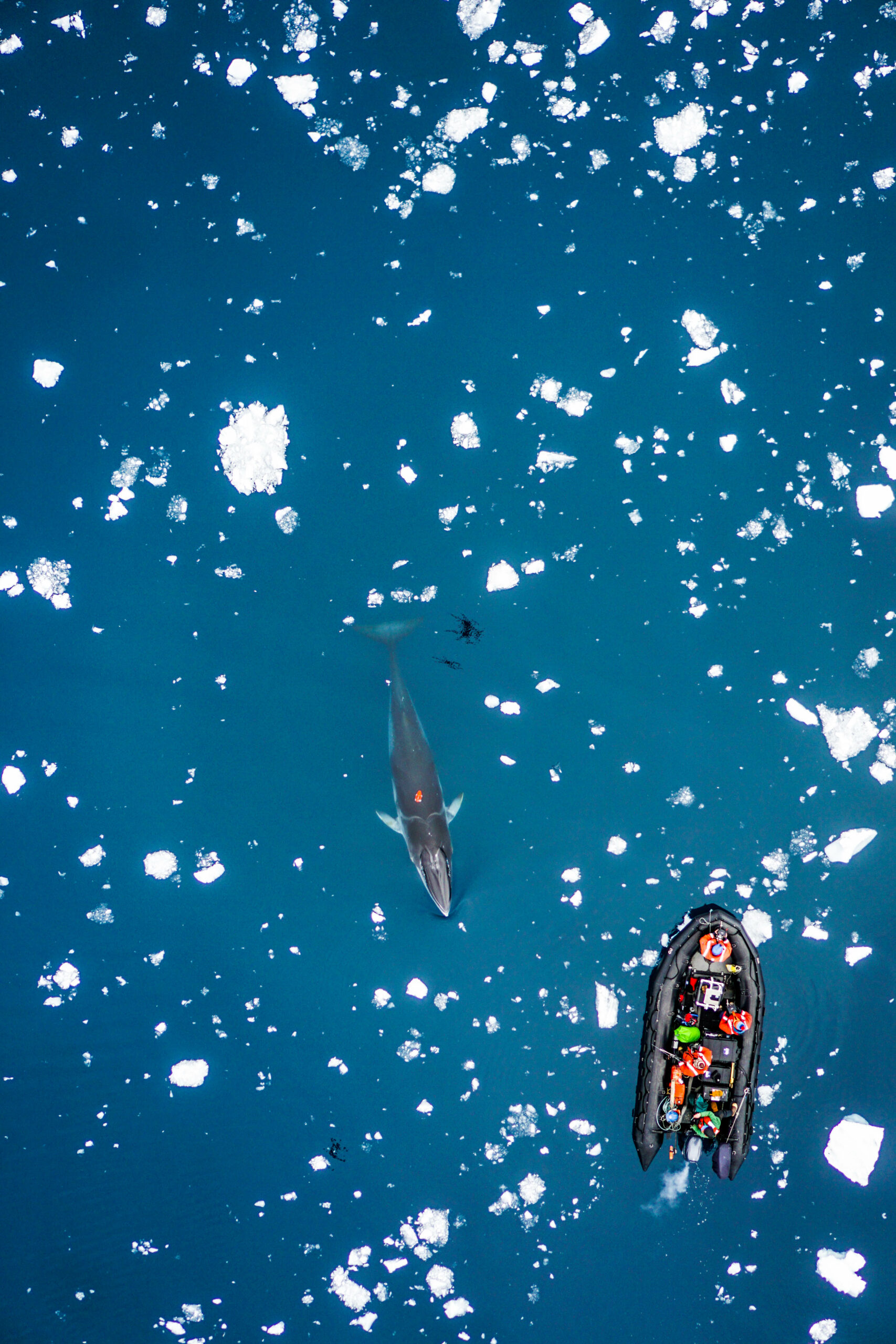
One of the many components of the SAPPHIRE Project is to understand how foraging success of blue whales is influenced by environmental variation (see this recent blog written by Dr. Dawn Barlow introducing each component of the project). When you cannot go to a grocery store or restaurant any time you are hungry, you must rely on stored energy from previous feeds to fuel energy needs. Body condition reflects an individual’s stored energy in the body as a result of feeding and thus represents the foraging success of an individual, which can then affect its potential for reproductive output and the individual’s overall health (see this previous blog). As discussed in a previous blog, drones serve as a valuable tool for obtaining morphological measurements of whales to estimate their body condition. We are using drones to collect aerial imagery of pygmy blue whales to obtain body condition measurements late in the foraging season between years 2024 and 2026 of the SAPPHIRE Project (Figure 2). We are quantifying body condition as Body Area Index (BAI), which is a relative measure standardized by the total length of the whale and well suited for comparing individuals and populations (Figure 3).
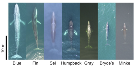
The GEMM Lab recently published an article led by Dr. Dawn Barlow where we investigated the differences in BAI between three blue whale populations: Eastern North Pacific blue whales feeding in Monterey Bay, California; Chilean blue whales feeding in the Corcovado Gulf; and New Zealand Pygmy blue whales feeding in the STB (Barlow et al., 2023). These three populations are interesting to compare since blue whales that feed in Monterey Bay and Corcovado Gulf migrate to and from these seasonally productive feeding grounds, while the Pygmy blue whales stay in Aotearoa New Zealand year-round. Interestingly, the Pygmy blue whales had higher BAI (were fatter) compared to the other two regions despite relatively lower productivity in their foraging grounds. This difference in body condition may be due to different life history strategies where the non-migratory Pygmy blue whales may be able to feed as opportunities arrive, while the migratory strategies of the Eastern North Pacific and Chilean blue whales require good timing to access high abundant prey. Another interesting and unexpected result from our blue whale comparison was that Pygmy blue whales are not so “pygmy”; they are actually the same size as Eastern North Pacific and Chilean blue whales, with an average size around 22 m. Our findings from this blue whale comparison leads us to more questions about how environmental conditions that vary from year to year influence body condition and reproduction of these “not so pygmy” blue whales.


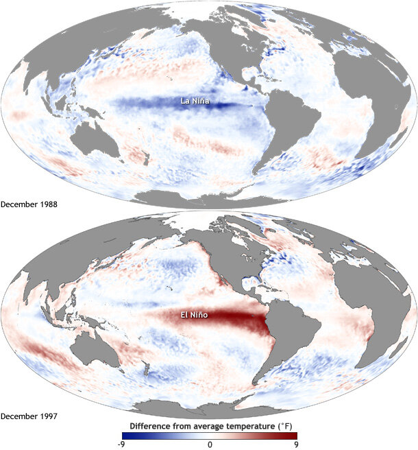
The GEMM Lab has been studying this population of Pygmy blue whales in the STB since 2013 and found that years designated as a marine heatwave resulted with a reduction in blue whale feeding activity. Interestingly, breeding activity is also reduced during marine heatwaves in the following season when compared to the breeding season following a more productive, typical foraging season. These findings indicate that fluctuations in the environment, such as marine heatwaves, may affect not only foraging success, but also reproduction in Pygmy blue whales.
To help us better understand reproductive patterns across years, we will use body width measurements from drone images paired with hormone concentrations collected from fecal and biopsy samples to identify pregnant individuals. Progesterone is a hormone secreted in the ovaries of mammals during the estrous cycle and gestation, making it the predominant hormone responsible for sustaining pregnancy. Recently, the GEMM Lab’s Dr. Alejandro Fernandez-Ajo wrote a blog discussing his publication identifying pregnant individual gray whales using drone-based body width measurements and progesterone concentrations from fecal samples (Fernandez et al., 2023). While individuals that were pregnant had higher levels of progesterone compared to when they were not pregnant, the body width at 50% of the body length served as a more reliable method for detecting pregnancy in gray whales. We will use similar methods to help identify pregnancy in Pygmy blue whales for the SAPPHIRE Project where will we examine body width measurement paired with progesterone concentrations collected from fecal and biopsy samples to identify pregnant individuals. We hope our work will help to better understand how climate change will influence Pygmy blue whale body condition and reproduction, and thus the overall health and resiliency of the population. Stay tuned!
References
Barlow, D. R., Bierlich, K. C., Oestreich, W. K., Chiang, G., Durban, J. W., Goldbogen, J. A., Johnston, D. W., Leslie, M. S., Moore, M. J., Ryan, J. P., & Torres, L. G. (2023). Shaped by Their Environment: Variation in Blue Whale Morphology across Three Productive Coastal Ecosystems. Integrative Organismal Biology, 5(1). https://doi.org/10.1093/iob/obad039
Fernandez Ajó, A., Pirotta, E., Bierlich, K. C., Hildebrand, L., Bird, C. N., Hunt, K. E., Buck, C. L., New, L., Dillon, D., & Torres, L. G. (2023). Assessment of a non-invasive approach to pregnancy diagnosis in gray whales through drone-based photogrammetry and faecal hormone analysis. Royal Society Open Science, 10(7), 230452. https://doi.org/10.1098/rsos.230452