Wavelet analysis to describe biological cycles and signals of non-stationarity

By Allison Dawn, GEMM Lab Master’s student, OSU Department of Fisheries, Wildlife, and Conservation Sciences, Geospatial Ecology of Marine Megafauna Lab 

During my second term of graduate school, I have been preparing to write my research proposal. The last two months have been an inspiring process of deep literature dives and brainstorming sessions with my mentors. As I discussed in my last blog, I am interested in questions related to pattern and scale (fine vs. mesoscale) in the context of the Pacific Coast Feeding Group (PCFG) of gray whales, their zooplankton prey, and local environmental variables.

My work currently involves exploring which scales of pattern are important in these trophic relationships and whether the dominant scale of a pattern changes over time or space. I have researched which analysis tools would be most appropriate to analyze ecological time series data, like the impressive long-term dataset the GEMM lab has collected in Port Orford as part of the TOPAZ  project, where we have monitored the abundance of whales and zooplankton, as well as environmental variables since 2016. 

A useful analytical tool that I have come across in my recent coursework and literature review is called wavelet analysis. Importantly, wavelet analysis can handle non-stationarity and edge detection in time series data. Non-stationarity is when a dataset’s mean and/or variance can change over time or space, and edge detection is the identification of the change location (in time or space). For example, it is not just the cycles or “ups and downs” of zooplankton abundance I am interested in, but when in time or where in space these cycles of “ups and downs” might change in relation to what their previous values, or distances between values, were. Simply stated, non-stationarity is when what once was normal is no longer normal. Wavelet analysis has been applied across a broad range of fields, such as environmental engineering (Salas et al. 2020), climate science (Slater et al. 2021), and bio-acoustics (Buchan et al. 2021). It can be applied to any time series dataset that might violate the traditional statistical assumption of stationarity. 

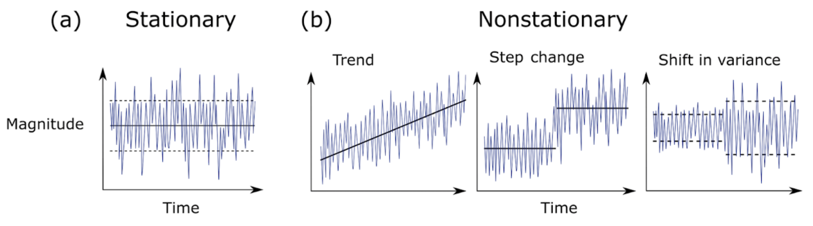
In a recent review of climate science methodology, Slater et al. (2021) outlined the possible behavior of time series data. Using theoretical plots, the authors show that data can a) have the same mean and variance over time, or b) have non-stationarity that can be broken into three major groups – trend, step change, or shifts in variance. Figure 1 further demonstrates the difference between stationary vs. non-stationary data in relation to a given variable of interest over time. 

Figure 1. Plots showing the possible magnitude of a given variable across a time series: a) Stationary behavior, b) Non-stationary trend, step-change, and a shift in variance. [Taken from Slater et. al (2021)].

Traditional correlation statistics assumes stationarity, but it has been shown that ecological time series are often non-stationary at certain scales (Cazelles & Hales, 2006). In fact, ecological data rarely meets the requirements of a controlled experiment that traditional statistics require. This non-stationarity of ecological data means that while widely-used methods like generalized linear models and analyses of variances (ANOVAs) can be helpful to assess correlation, they are not always sufficient on their own to describe the complex natural phenomena ecologists seek to explain. Non-stationarity occurs frequently in ecological time series, so it is appropriate to consider analysis tools that will allow us to detect edges to further investigate the cause.

Wavelet analysis can also be conducted across a time series of multiple response variables to assess if these variables share high common power (correlation). When data is combined in this way it is called a cross-wavelet analysis. An interesting paper used cross-wavelet analysis to assess the seasonal response of zooplankton life history in relation to climate warming (Winder et. al 2009). Results from their cross-wavelet analysis showed that warming temperatures over the past two decades increased the voltinism (number of broods per year) of copepods. The authors show that where once annual recruitment followed a fairly stationary pattern, climate warming has contributed to a much more stochastic pattern of zooplankton abundance. From these results, the authors contribute to the hypothesis that climate change has had a temporal impact on zooplankton population dynamics, and recruitment has increasingly drifted out of phase from the original annual cycles. 

Figure 2. Cross-wavelet spectrum for immature and adult Leptodiaptomus ashlandi for 1965 through either 2000 or 2005. Plots show a) immatures and temperature, b) adults and temperature, c) immatures and phytoplankton, and d) adults and phytoplankton. Arrows indicate phase between combined time series. 0 degrees is in-phase and 180 degrees is anti-phase. Black contour lines show “cone of influence” or the 95% significance level, every value within the cone is considered significant. Left axis shows the temporal period, and the color legend shows wavelet frequency power, with low frequencies in blue and high frequencies in red. Plots show strong covariation of high common power at the 12-month period until the 1980s. This pattern is especially evident in plot c) and d). [Taken from (Winder et. al 2009)].

While wavelet and cross-wavelet analyses should not be the only tool used to explore data, due to its limitations with significance testing, it is still worth implementing to gain a better understanding of how time series variables relate to each other over multiple spatial and/or temporal scales. It is often helpful to combine multiple methods of analysis to get a larger sense of patterns in the data, especially in spatio-temporal research.

When conducting research within the context of climate change, where the concentration of CO2 in ppm in the atmosphere is a non-stationary time series itself (Figure 3), it is important to consider how our datasets might be impacted by climate change and wavelet analysis can help identify the scales of change. 

Figure 3. Plot showing the historic fluctuations of CO^2 and the recent deviation from normal levels. Source: https://globalclimate.ucr.edu/resources.html

When considering our ecological time series of data in Port Orford, we want to evaluate how changing ocean conditions may be related to data trends. For example, has the annual mean or variance of zooplankton abundance changed over time, and where has that change occurred in time or space? These changes might have occurred at different scales and might be invisible at other scales. I am eager to see if wavelet analysis can detect these sorts of changes in the abundance of zooplankton across our time series of data, particularly during the seasons of intense heat waves or upwelling. 

Did you enjoy this blog? Want to learn more about marine life, research and conservation? Subscribe to our blog and get a weekly email when we make a new post! Just add your name into the subscribe box on the left panel.

References

Buchan, S. J., Pérez-Santos, I., Narváez, D., Castro, L., Stafford, K. M., Baumgartner, M. F., … & Neira, S. (2021). Intraseasonal variation in southeast Pacific blue whale acoustic presence, zooplankton backscatter, and oceanographic variables on a feeding ground in Northern Chilean Patagonia. Progress in Oceanography, 199, 102709.

Cazelles, B., & Hales, S. (2006). Infectious diseases, climate influences, and nonstationarity. PLoS Medicine, 3(8), e328.

Salas, J. D., Anderson, M. L., Papalexiou, S. M., & Frances, F. (2020). PMP and climate variability and change: a review. Journal of Hydrologic Engineering, 25(12), 03120002.

Slater, L. J., Anderson, B., Buechel, M., Dadson, S., Han, S., Harrigan, S., … & Wilby, R. L. (2021). Nonstationary weather and water extremes: a review of methods for their detection, attribution, and management. Hydrology and Earth System Sciences, 25(7), 3897-3935.

Winder, M., Schindler, D. E., Essington, T. E., & Litt, A. H. (2009). Disrupted seasonal clockwork in the population dynamics of a freshwater copepod by climate warming. Limnology and Oceanography, 54(6part2), 2493-2505.

Introducing IndividuWhale!

By Lisa Hildebrand, PhD student, OSU Department of Fisheries, Wildlife, & Conservation Sciences, Geospatial Ecology of Marine Megafauna Lab

If you are an avid reader of our blog, you probably know quite a bit about gray whales, specifically the Pacific Coast Feeding Group (PCFG) of gray whales. Of the just over 50 GEMM Lab blogs written in 2021, 43% of them were about PCFG gray whales (or at least mentioned gray whales in some way). I guess this statistic is not too surprising when you consider that six of the 10 GEMM Lab members conduct gray whale-related research. You might think that we would have reached our annual limit of online gray whale content with that many blogs featuring these gentle giants, but you would in fact be wrong…

At the end of 2021, we launched a brand new website all about gray whales called IndividuWhale! It features stories of some of the Oregon coast’s most iconic gray whales, as well as information about how we study them, stressors they experience in our waters, and even a game to test your gray whale identification skills. IndividuWhale is a true labor of love that took over a year to create and that we are extremely proud to share with you today. Before I tell you more about the website, I want to take a moment to give a huge shout out to Erik Urdahl who was instrumental in getting this website off the ground and making it as interactive and beautiful as it is – hurrah Erik!

Equal‘s right side with visible boat propeller scars. Source: GEMM Lab.

Like us humans, gray whales have individual personalities and stories. They experience life-altering events, go through periods of stress, must provide for their offspring, and can behave differently to one another. Since Leigh & co. have been conducting in-depth research about PCFG gray whales in Oregon waters since 2016, we have been able to document several fascinating stories and events that these individuals have experienced. Take Equal, for example, a male whale that is at least 7 years old. The GEMM Lab observed Equal on consecutive days in June 2018, where on the first day he looked healthy and normal, but on the second day had fresh boat propeller-like scars on his back. Not only did we document these scars in photographs, but we were also able to collect a fecal sample from Equal the day we observed him with these scars. After analyzing his fecal sample for stress hormones, we discovered that Equal had very high stress levels compared to previous samples collected – unsurprising seeing as he had been hit by a boat! While this event was certainly sad for Equal (although don’t worry – we have seen him many times again in the years after this event looking healthy & normal once again), it was a very fortuitous occurrence for us since we were able to “validate” our stress hormone data relative to the value from Equal when he was clearly stressed out. Find out more about Equal as well as seven other gray whales here!

You might be wondering, how we knew that the whale with the boat propeller scar was Equal and how we recognize him again years after the incident. Gray whales have unique pigmentation patterns on their bodies and flukes that allow us to re-identify individuals between years and distinguish them from one another. Additionally, scars, such as those that Equal now carries on his back, can also be useful in telling whales apart. Therefore, we take photographs of every whale we see to match markings and identify whales. This process is called photo ID. Some individuals can have very distinctive markings, such as Roller Skate who has two big white dots on her right side, while others can look more inconspicuous, like Clouds. Therefore, conducting photo ID requires a lot of attention to detail and perseverance. To learn more about the different features we use to identify individuals, check out the “Studying Whales With Photographs” page. Do you think you have what it takes to tell individuals apart? Then try your luck at our photo ID game after!

Test your photo ID skills in our whale match game!

Unfortunately, these whales do not live in a pristine environment, as is evidenced by Equal’s story. Their main objective during the summer when in Oregon waters is to gain weight (energy stores) by consuming large amounts of prey, which is made more difficult by a number of stressors, including potential fishery entanglements, ocean noise, vessel traffic, and habitat changes. We describe these four stressors on the IndividuWhale website since we are trying to assess the impacts of them on gray whales through our research, however they are certainly not the only stressors that these whales experience. Little is known about the level at which these stressors may have a negative impact on the whales, and how whales react when they experience some of these stressors in concert. The answers to these questions are difficult to tease apart but the GRANITE project is aiming to do so through a framework called Population Consequences of Multiple Stressors (read more about it here). This approach requires a lot of data on a lot of individuals in a population and as you can see from the IndividuWhale website, we are slowly starting to get there! 2022 will certainly bring many more gray whale-themed blogs to this website, and you can share in our journey of learning about the lives of PCFG gray whales by exploring the IndividuWhale website (https://www.individuwhale.com).

Social turmoil due to the approval of an offshore oil exploration project off the coast of Argentina.

Dr. Alejandro A. Fernández Ajó, Postdoctoral Scholar, Marine Mammal Institute – OSU Department of Fisheries, Wildlife, & Conservation Sciences, Geospatial Ecology of Marine Megafauna (GEMM) Lab.

I just returned to my home country, Argentina, after over 2 years without leaving the USA due to COVID-19 travel restrictions. Being back with my family, my friends, my culture, and speaking my native language feels great and relaxing. However, I returned to a country struggling to rebound from the coronavirus pandemic. I am afraid this post pandemic scenario places Argentina in a vulnerable situation. The need for economic growth could result in decisions or policies that, in the long term, hurt the country, leaving environmental damage for potential economic growth.

Argentina holds extensive oil and gas deposits, including the world’s second largest gas formation, Vaca Muerta. Although offshore (i.e., in the ocean) oil exploration and exploitation are not yet extensively developed, the intention of offshore gas and oil drilling is on the agenda. In July 2021, a public hearing was held with the purpose to consider the environmental impact assessment for carrying out seismic exploration in the North Argentinian basin off the southern coast of the Buenos Aires province. Over 90% of the participants, including scientists, researchers, technicians from various institutions, non-governmental organizations and representatives of the fishing sector spoke against the project and highlighted the negative impacts that such activity can generate on marine life, and to other socioeconomic activities such as tourism and fishing, not only in Argentina but at the regional level.

Thousands of people marched along the beaches and the main coastal cities of Argentina to protest against the approval for a seismic explorations project in the Argentinian basin. Photo source: prensaobrera.com

Seismic prospections are usually done with the purpose for oil and gas exploitation and less frequently for research purposes. In seismic prospections, ships carry out explosions with airguns, whose sound waves reach the seabed, bounce back and are captured by receivers on the ships to map the petroleum deposits in seafloor and identify potential areas for hydrocarbon extractions. The sound emitted by the seismic airguns can reach extremely loud levels of sounds that travel for thousands of miles underwater. Such extreme high levels of sound can alter the behavior of many marine species, from the smallest planktonic species, to the largest marine mammals, masking their communication, causing physical and physiological stress, interfering with their vital functions, and reducing the local availability of prey (Di Iorio & Clark, 2010; Hildebrand, 2009; Weilgart, 2018).

Here you can listen to a short audio clip of a seismic airgun firing every ~8 seconds, a typical pattern. Close your eyes and imagine you are a whale living in this environment. Now, put the clip on loop and play it for three months straight. This would be the soundscape that whales living in a region of oil and gas exploration hear, as seismic surveys often last 1-4 months (see our previous post “Hearing is believing” for more details).

Despite the public rejection and the mounting evidence about the negative impacts and environmental risks associated with such activities, the government approved the initiation of the seismic prospection off the southern coast of Buenos Aires. In response, thousands of people marched along the beaches and the main coastal cities of Argentina to protest against the oil exploration project. The areas where the seismic surveys will be carried out overlap largely with the southern right whale’s migration routes and feeding areas during their spring and summer (Figure 1). Likewise, the area overlaps with highly productive areas in the ocean that hosts great biodiversity of species of ecological and commercial importance, including the feeding areas of seabirds, turtles and other marine mammals. Additionally, the seismic activity will endanger the health of the beaches of the coast of Buenos Aires and Uruguay where thousands of tourists spend the summer to escape from the large cities.

Figure 1. The map on the left is showing (light blue squares CAN_100, CAN_108, and CAN_114) the areas where seismic prospections are proposes. The map on the right is showing the individual satellite track lines for eleven individual southern right whales (SRW) during the feeding season. You can observe that the proposed area for seismic explorations overlaps with critical feeding habitat for the SRW. Source: Whale Conservation Institute of Argentina (ICB).

The impacts of these activities to marine wildlife are difficult to control and monitor (Elliott et al. 2019, Gordon et al, 2003), especially for large whales that are a very challenging taxa to study (Hunt et al. 2013). We know that the ability to perceive biologically important sounds is critical to marine mammals, and acoustic disturbance through human-generated noise can interfere with their natural functions. Sounds from seismic surveys are intense and have peak frequency bands overlapping those used by baleen whales (Di Lorio & Clark, 2010); however, evidence of interference with baleen whale acoustic communication, and the effects on their health and physiology are sparse. In this context, the GEMM Lab project GRANITE (Gray Whale Response to Ambient Noise Informed by Technology and Ecology), plans to generate information to fulfill these knowledge gaps and provide tools to aid conservation and management decisions in terms of allowable noise level in whale habitats. I am hopeful such information will reach decision makers and influence their decisions, however, sometimes it is frustrating to see how evidence-based information generated with high quality standards are often ignored.

The recent approval of the seismic exploration in Argentina is an example of my frustration. There is no way that the oil industry can guarantee a low-risk of impact on biodiversity and the environment. There are too many examples of environmental catastrophes related to the oil industries at sea that speak for themselves. Moreover, the promotion of such activities goes against the compromises assumed by the country to work to mitigate the effects of Climate Change, and to achieve the reductions of the greenhouse gas emissions to comply with the Paris Agreement. Decades of research help recognized the areas that would be impacted by these seismic activities as key habitat for the life cycle of whales, penguins, seals and more. But, apparently all these scientific data are ignored at the time of weighing the tradeoffs between “economic development” and environmental impacts. As a conservation biologist, I am questioning what can be done in order to be heard and significantly influence such decisions.

Did you enjoy this blog? Want to learn more about marine life, research, and conservation? Subscribe to our blog and get a weekly alert when we make a new post! Just add your name into the subscribe box on the left panel.

References:

  • Di Iorio, L., & Clark, C. W. (2010). Exposure to seismic survey alters blue whale acoustic communication. Biology Letters, 6(1), 51–54. https://doi.org/10.1098/rsbl.2009.0651
  • Weilgart, L. (2018). The impact of ocean noise pollution on fish and invertebrates. Report for OceanCare, Switzerland.
  • Elliott, B. W., Read, A. J., Godley, B. J., Nelms, S. E., & Nowacek, D. P. (2019). Critical information gaps remain in understanding impacts of industrial seismic surveys on marine vertebrates. In Endangered Species Research (Vol. 39, pp. 247–254). Inter-Research. https://doi.org/10.3354/esr00968
  • Gordon, J., Gillespie, D., Potter, J., Frantzis, A., Simmonds, M. P., Swift, R., & Thompson, D. (2003). A review of the effects of seismic surveys on marine mammals. Marine Technology Society Journal37(4), 16-34.
  • Hunt, K. E., Moore, M. J., Rolland, R. M., Kellar, N. M., Hall, A. J., Kershaw, J., Raverty, S. A., Davis, C. E., Yeates, L. C., Fauquier, D. A., Rowles, T. K., & Kraus, S. D. (2013). Overcoming the challenges of studying conservation physiology in large whales: a review of available methods. Conservation Physiology, cot006–cot006. https://doi.org/10.1093/conphys/cot006

Drones with lasers: almost as cool as “sharks with laser beams attached to their heads”

Dr. KC Bierlich, Postdoctoral Scholar, OSU Department of Fisheries, Wildlife, & Conservation Sciences, Geospatial Ecology of Marine Megafauna (GEMM) Lab

The recent advancement in drones (or unoccupied aircraft systems, UAS) has greatly enhanced opportunities for scientists across a broad range of disciplines to collect high-resolution aerial imagery. Wildlife researchers in particular have utilized this technology to study large elusive animals, such as whales, to observe their behavior (see Clara Bird’s blog) and obtain morphological measurements via photogrammetry (see previous blog for a brief history on photogrammetry and drones). However, obtaining useful measurement data is not as easy as flying the drone and pressing record. For this blog, I will provide a brief overview on the basics of using photogrammetry to extract morphological measurements from images collected with drones, as well as the associated uncertainty from using different drone platforms. 

During my PhD at Duke University, I co-developed an open-source photogrammetry software called MorphoMetriX to measure whales in images I collected using drones (Fig. 1) (Torres and Bierlich, 2020) (see this blog for some fieldwork memoirs!). The software is designed to be flexible, simple to use, and customizable without knowledge of scripting languages. Using MorphoMetriX, measurements are made in pixels and then multiplied by the ground sampling distance (GSD) to convert to standard units (e.g., meters) (Fig. 2A). GSD represents the distance on the ground each pixel represents (i.e., the linear size of the pixel) and therefore sets the scale of the image (i.e., cm per pixel). Figure 2A describes how GSD is dependent on the camera sensor, focal length lens, and altitude. Thus, drones equipped with different cameras and focal length lenses will have inherent differences in GSD as altitude increases (Fig. 2B). A larger GSD increases the length each pixel represents in a photo and results in a lower resolution image, potentially obscuring important features in the photo and introducing measurement error.

Figure 1. An example of a Pacific Coast Feeding Group gray whale measured in MorphoMetriX (Torres & Bierlich, 2020).
Figure 2: Overview of photogrammetry methods and calculating ground sampling distance (GSD). A) Photogrammetry methods for how each image is scaled to convert measurements in pixels to standard units (e.g., meters). Altitude is the distance between the camera lens and whale (usually at the surface of the water). Figure from Torres and Bierlich (2020). B) The exact (not accounting for distortion or altitude error) ground sampling distance (GSD) for two drone platforms commonly used to obtain morphological measurements of cetaceans. The difference in GSD between the P4Pro and Inspire 1 is due to the difference in sensor width and focal lengths of the cameras used. Figure from Bierlich et al. (2021).

Obtaining accurate altitude information is a key component in obtaining accurate measurements. All drones are equipped with a barometer, which measures altitude from changes in pressure. In general, barometers usually yield low accuracy in the altitude recorded, particularly for low-cost sensors commonly found on small, off-the-shelf drones (Wei et al., 2016). Dawson et al. (2017) added a laser altimeter (i.e., LightWare SF11/C, https://www.mouser.com//datasheet//2//321//28054-SF11-Laser-Altimeter-Manual-Rev8-1371857.pdf) to a drone, which yields higher accuracy in the altitude recorded. Since then, several studies have adopted use of a laser altimeter to study different species of baleen whales (i.e., Gough et al., 2019; Christiansen et al., 2018).

The first chapter of my dissertation, which was published last year in Marine Ecology Progress Series, compared the accuracy of several drones equipped with different camera sensors, focal length lenses, and a barometer vs. laser altimeter (Bierlich et al., 2021). We flew each drone over a known sized object floating at the surface and collected images at various altitudes (between 10 – 120 m). We used the known size of the floating object to determine the percent error of each measurement at each altitude. We found that 1) there is a lot of variation in measurement error across the different drones when using a barometer to measure altitude and 2) using a laser altimeter dramatically reduces measurement error for each drone (Fig. 3).

Figure 3. The % error for measurements from different drones. Black dashed line represents 0% error (true length = 1.48 m). The gray dashed lines represent under- and over-estimation of the true length by 5% (1.41 and 1.55 m, respectively).

These findings are important because if a study is analyzing measurements that are from more than one drone, the uncertainty associated with those measurements must be taken into account to know if measurements are reliable and comparable. For instance, let’s say we are comparing the body length of two different populations and found that population A is significantly longer than population B. From looking at Figure 3, that significant difference in length between population A and B could be unreliable as the difference may be due to the bias introduced by the type of drone, camera sensor, focal length lens, and whether a barometer or laser altimeter was used for recording altitude. In other words, without incorporating uncertainty associated with each measurement, how do you trust your measurement? 

Hence, the National Institute of Standards and Technology (NIST) states that a measurement is complete only when accompanied by a quantitative statement of its uncertainty (Taylor & Kuyatt, 1994). In our Bierlich et al. (2021) study, we develop a Bayesian statistical model where we use the measurements of the known-sized object floating at the surface (what was used for Fig. 3) as training data to predict the lengths of unknown-sized whales. This Bayesian approach views data and the underlying parameters that generated the data (such as the mean or standard deviation) as random, and thus can be described by a statistical distribution. Using Bayes’ Theorem, a model of the observed data (called the likelihood function), is combined with prior knowledge pertaining to the underlying parameters (called the prior probability distribution) to form the posterior probability distribution, which serves as updated knowledge about the underlying parameter. For example, if someone told me they saw a 75 ft blue whale, I would not be phased. But if someone told me they saw a 150 ft blue whale, I would be skeptical – I’m using prior knowledge to determine the probability of this statement being true. 

The posterior probability distribution produced by this Bayesian approach can also serve as new prior information for subsequent analyses. Following this framework, we used the known-sized objects to first estimate the posterior probability distribution for error for each drone. We then used that posterior probability distribution for error specific to each drone platform as prior information to form a posterior predictive distribution for length of unknown-sized whales. The length of an individual whale can then be described by the mean of this second posterior predictive distribution, and its uncertainty defined as the variance or an interval around the mean (Fig. 4). 

Figure 4. An example of a posterior predictive distribution for total length of an individual blue whale. The black bars represent the uncertainty around the mean value (the black dot) – the longer black bars represent the 95% highest posterior density (HPD) interval, and the shorter black bars represent the 65% HPD interval. 

For over half a decade, the GEMM Lab has been collecting drone images of Pacific Coast Feeding Group (PCFG) of gray whales off the coast of Oregon to measure their morphology and body condition (see GRANITE Project Blog). We have been using several different types of drones equipped with different cameras, focal length lenses, barometers, and laser altimeters. These measurements from different drones will inherently have different levels of error associated with them, so adapting these methods for incorporating uncertainty will be key to ensure our measurements are comparable and analyses are robust. To do this, we fly over a known-sized board (1 m) at the start of each flight to use as training data to generate a posterior predictive distribution for length of the an unknown-sized PCFG gray whale that we fly over (Fig. 5). Likewise, we are working closely with several other collaborators who are also using different drones. Incorporating measurement uncertainty from drones used across research labs and in different environments will help ensure robust analyses and provide great opportunity for some interesting comparisons – such as differences in gray whale body condition on their feeding grounds in Oregon vs. their breeding grounds in Baja, Mexico, and morphological comparisons with other baleen whale species, such as blue and humpback whales. We are currently wrapping up measurement from thousands of boards (Fig. 5) and whales (Fig. 1) from 2016 – 2021, so stay tuned for the results!

Figure 5. An example of a known-sized object (1 m long board) used as training data to assess measurement uncertainty. 

References

Bierlich, K.C., Schick, R.S., Hewitt, J., Dale, J., Goldbogen, J.A., Friedlaender, A.S., Johnston D.J. (2021). A Bayesian approach for predicting photogrammetric uncertainty in morphometric measurements derived from UAS. Marine Ecology Progress Series. DOI: https://doi.org/10.3354/meps13814

Christiansen F, Vivier F, Charlton C, Ward R, Amerson A, Burnell S, Bejder L (2018) Maternal body size and condition determine calf growth rates in southern right whales. Mar Ecol Prog Ser 592: 267−281

Dawson SM, Bowman MH, Leunissen E, Sirguey P (2017) Inexpensive aerial photogrammetry for studies of whales and large marine animals. Front Mar Sci 4: 366

Gough, W.T., Segre, P.S., Bierlich, K.C., Cade, D.E., Potvin, J., Fish, F. E., Dale, J., di Clemente, J., Friedlaender, A.S., Johnston, D.W., Kahane-Rapport, S.R., Kennedy, J., Long, J.H., Oudejans, M., Penry, G., Savoca, M.S., Simon, M., Videsen, S.K.A., Visser, F., Wiley, D.N., Goldbogen, J.A. (2019). Scaling of swimming performance in baleen whales. Journal of Experimental Biology222(20).https://doi.org/10.1242/jeb.204172  

Taylor, B. N., and Kuyatt, C. E. (1994). Guidelines for Evaluating and Expressing the Uncertainty of NIST Measurement Results. Washington, DC: National Institute of Standards and Technology. 1–25.

Torres, W.I., & Bierlich, K.C. (2020). MorphoMetriX: a photogrammetric measurement GUI for morphometric analysis of megafauna. Journal of Open Source Software5(45), 1825. https://doi.org/10.21105/joss.01825  

Wei S, Dan G, Chen H (2016) Altitude data fusion utilizing differential measurement and complementary filter. IET Sci Meas Technol (Singap) 10: 874−879