By Lisa Hildebrand, PhD candidate, OSU Department of Fisheries, Wildlife, & Conservation Sciences, Geospatial Ecology of Marine Megafauna Lab
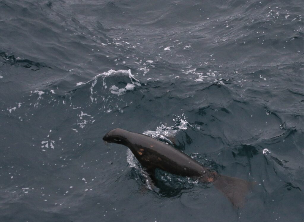
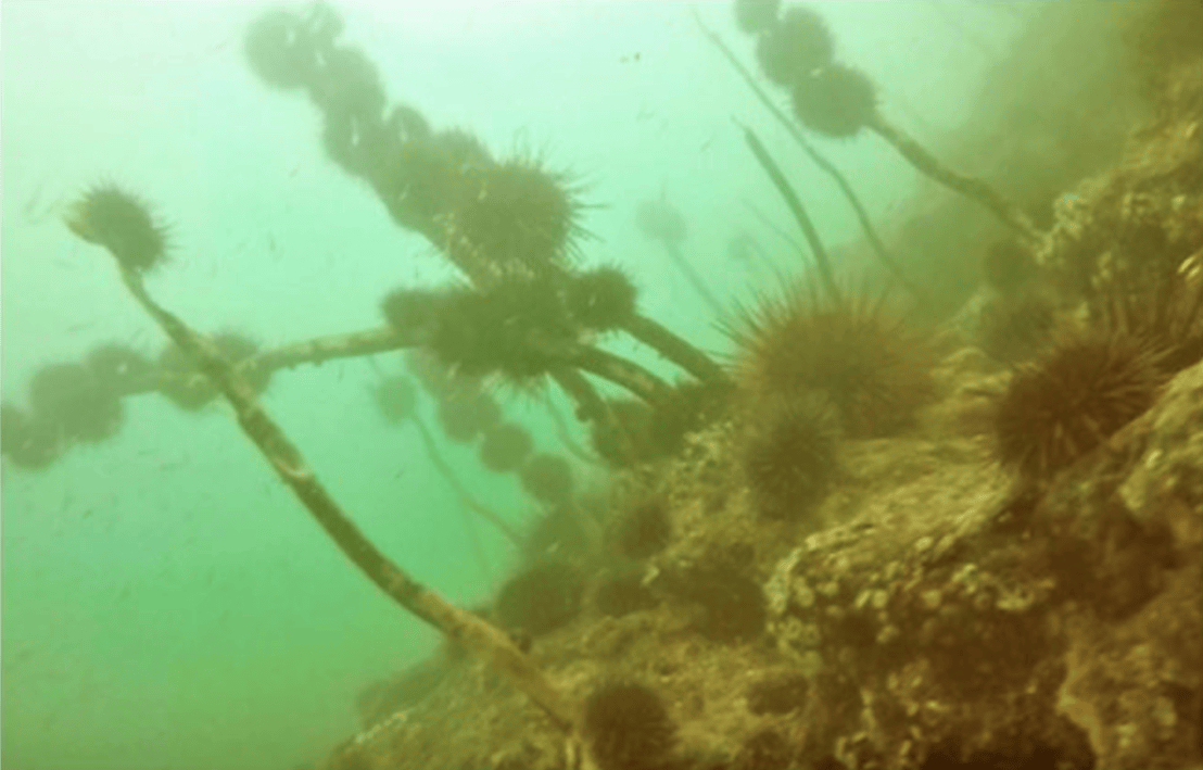
As many of our avid readers already know, the Pacific Coast Feeding Group (PCFG) of gray whales employs a wide range of foraging tactics to feed on a number of different prey items in various benthic substrate types (Torres et al. 2018). One example foraging tactic is when PCFG whales, particularly when they are in the Oregon portion of their feeding range, forage on mysid shrimp in and near kelp beds on rocky reefs. We have countless drone video clips of whales weaving their large bodies through kelp and many photographs of whales coming to the surface to breath completely covered in kelp, looking more like a sea monster than a whale (Figure 1). So, when former intern Dylan Gregory made an astute observation during the 2018 TOPAZ/JASPER field season in Port Orford about a GoPro video the field team collected that showed many urchins voraciously feeding on an unhealthy-looking kelp stalk (Figure 2a), it made us wonder if and how changes to kelp forests may impact gray whales.

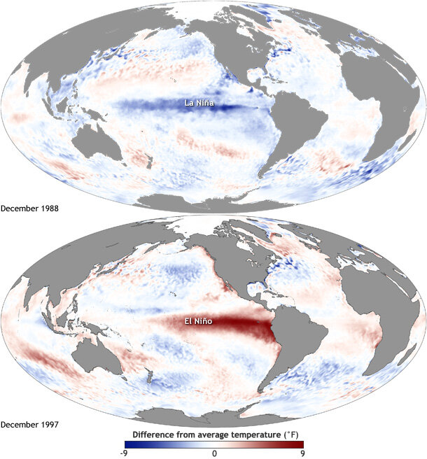
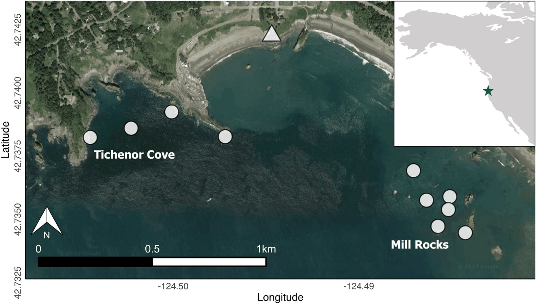
Kelp forests are widely used as a marine example of trophic cascades. Trophic cascades are trigged by the addition/removal of a top predator to/from a system, which causes changes further down the trophic chain. Sea urchins are common inhabitants of kelp forests and in a balanced, healthy system, urchin populations are regulated by predators as they behave cryptically by hiding in crevices in the reef and individual urchins feed passively on drift kelp that breaks off from larger plants. When we think about who controls urchins in kelp forests, we probably think of sea otters first. However, sea otters have been absent from Oregon waters for over a century (Kone et al. 2021), so who controls urchins here? The answer is the sunflower sea star (Figure 2b). Sunflower sea stars are large predators with a maximum arm span of up to 1 m! Unfortunately, a disease epidemic that started in 2013 known as sea star wasting disease caused 80-100% population decline of sunflower sea stars along the coastline between Mexico and Alaska (Harvell et al. 2019). Shortly thereafter, a record-breaking marine heatwave caused warm, nutrient-poor water conditions to persist in the northeast Pacific Ocean from 2014 to 2016 (Jacox et al. 2018). These co-occurring stressors caused unprecedented and long-lasting decline of a previously robust kelp forest in northern California (Rogers-Bennett & Catton 2019), where sea otters are also absent. Given the biogeographical similarity between southern Oregon and northern California and the observation made by Dylan in 2018, we decided to undertake an analysis of the eight years of data collected during the TOPAZ/JASPER project in Port Orford starting in 2016, to investigate the trends of four trophic levels (purple sea urchins, bull kelp, zooplankton, and gray whales) across space and time. The results of our study were published last week in Scientific Reports and I am excited to be able to share them with you today.

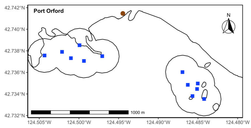
Every day during the TOPAZ/JASPER field season, two teams head out to collect data. One team is responsible for tracking gray whales from shore using a theodolite, while the other team heads out to sea on a tandem research kayak to collect prey data (Figure 3). The kayak team samples prey in multiple ways, including dropping a GoPro camera at each sampling station. When the project was first developed, the original goal of these GoPro videos was to measure the relative abundance of prey. Since the sampling stations occur on or near reefs that are shallow with dense surface kelp, traditional methods to assess prey density, such as using a boat with an echosounder, are not suitable options. Instead, GEMM Lab PI Leigh Torres, together with the first Master’s student on this project Florence Sullivan, developed a method to score still images extracted from the GoPro videos to estimate relative zooplankton abundance. However, after we saw those images of urchins feeding on kelp in 2018, we decided to develop another protocol that allowed us to use these GoPro videos to also characterize sea urchin coverage and kelp condition. Once we had occurrence values for all four species, we were able to dig into the spatiotemporal trends.
When we examined the trends for each of the four study species across years, we found that purple sea urchin coverage in both of our study sites within Port Orford increased dramatically within our study period (Figure 4). In 2016, the majority of our sampled stations contained no visible urchins. However, by 2020, we detected urchins at every sampling station. For kelp, we saw the reverse trend; in 2016 all sampling stations contained kelp that was healthy or mostly healthy. But by 2019, there were many stations that contained kelp in poor health or where kelp was absent entirely. Zooplankton and gray whales experienced similar temporal trends as the kelp, with their occurrence metrics (abundance and foraging time, respectively) having higher values at the start of our study period and declining steadily during the eight years. While the rise in urchin coverage across our study area occurred concurrently with the decrease in kelp condition, zooplankton abundance, and gray whale foraging, we wanted to explicitly test how these species are related to one another based on prior ecological knowledge.

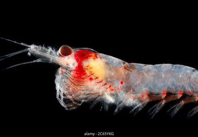
To test whether urchin coverage had an effect on kelp condition, we hypothesized that increased urchin coverage would be correlated with reduced kelp condition based on the decades of research that has established a negative relationship between the two when a trophic cascade occurs in kelp forest systems. Next, we wanted to test whether kelp condition had an effect on zooplankton abundance and hypothesized that increased kelp condition would be correlated with increased zooplankton abundance. We based this hypothesis on several pieces of prior knowledge, particularly as they pertain to mysid shrimp: (1) high productivity within kelp beds provides food for mysids, including kelp zoospores (VanMeter & Edwards 2013), (2) current velocities are one third slower inside kelp beds compared to outside (Jackson & Winant 1983), which might support the retention of mysids within kelp beds since they are not strong swimmers, and (3) the kelp canopy may serve as potential protection for mysids from predators (Coyer 1984). Finally, we wanted to test whether both kelp condition and zooplankton abundance have an effect on gray whales and we hypothesized that increased values for both would be correlated with increased gray whale foraging time. While the reasoning behind our hypothesized correlation between zooplankton prey and gray whales is obvious (whales eat zooplankton), the reasoning behind the kelp-whale connection may not be. We speculated that since kelp habitat may aggregate or retain zooplankton prey, gray whales may use kelp as an environmental cue to find prey patches.
When we tested our hypotheses through generalized additive models, we found that increased urchin coverage was significantly correlated with decreased kelp condition in both study sites, providing evidence that a shift from a kelp forest to an urchin barren may have occurred in the Port Orford area. Additionally, increased kelp condition was correlated with increased zooplankton abundance, supporting our hypothesis that kelp forests are an important habitat and resource for nearshore zooplankton prey. Interestingly, this relationship was bell-shaped in one of our two study sites, suggesting that there are other factors besides healthy bull kelp that influence zooplankton abundance, which likely include upwelling dynamics, habitat structure, and local oceanographic characteristics. For the whale model, we found that increased kelp condition was significantly correlated with increased gray whale foraging time, which may corroborate our hypothesis that gray whales use kelp as an environmental cue to locate prey. Zooplankton abundance was significantly correlated with gray whale foraging time in one of our two sites. Once again, this relationship was bell-shaped, which suggests other factors influence gray whale foraging time, including prey quality (Hildebrand et al. 2022) and density.

Our results highlight the potential larger impacts of reduced gray whale foraging time as a result of these trophic dynamics may cause at the individual and population level. If an area that was once a reliable source of food (like Port Orford) is no longer favorable, then whales likely search for other areas in which to feed. However, if the areas affected by these dynamics are widespread, then individuals may spend more time searching for, and less time consuming, prey, which could have energetic consequences. While our study took place in a relatively small spatial area, the trophic dynamics we documented in our system may be representative of patterns across the PCFG range, given ecological and topographic similarities in habitat use patterns. In fact, in the years with the lowest kelp, zooplankton, and whale occurrence (2020 and 2021) in Port Orford, the GRANITE field team also noted low whale numbers and minimal surface kelp extent in the central Oregon field site off of Newport. However, ecosystems are resilient. We are hopeful that the dynamics we documented in Port Orford are just short-term changes and that the system will return to its former balanced state with less urchins, more healthy bull kelp, zooplankton, and lots of feeding gray whales.
If you are interested in getting a more detailed picture of our methods and analysis, you can read our open access paper here: https://www.nature.com/articles/s41598-024-59964-x
Did you enjoy this blog? Want to learn more about marine life, research, and conservation? Subscribe to our blog and get a weekly message when we post a new blog. Just add your name and email into the subscribe box below.
References
Coyer, J. A. (1984). The invertebrate assemblage associated with the giant kelp, Macrocystis pyrifera, at Santa Catalina Island, California: a general description with emphasis on amphipods, copepods, mysids, and shrimps. Fishery Bulletin, 82(1), 55-66.
Harvell, C. D., Montecino-Latorre, D., Caldwell, J. M., Burt, J. M., Bosley, K., Keller, A., … & Gaydos, J. K. (2019). Disease epidemic and a marine heat wave are associated with the continental-scale collapse of a pivotal predator (Pycnopodia helianthoides). Science advances, 5(1), eaau7042.
Hildebrand, L., Sullivan, F. A., Orben, R. A., Derville, S., & Torres, L. G. (2022). Trade-offs in prey quantity and quality in gray whale foraging. Marine Ecology Progress Series, 695, 189-201.
Jackson, G. A., & Winant, C. D. (1983). Effect of a kelp forest on coastal currents. Continental Shelf Research, 2(1), 75-80.
Jacox, M. G., Alexander, M. A., Mantua, N. J., Scott, J. D., Hervieux, G., Webb, R. S., & Werner, F. E. (2018). Forcing of multi-year extreme ocean temperatures that impacted California Current living marine resources in 2016. Bull. Amer. Meteor. Soc, 99(1).
Kone, D. V., Tinker, M. T., & Torres, L. G. (2021). Informing sea otter reintroduction through habitat and human interaction assessment. Endangered Species Research, 44, 159-176.
Rogers-Bennett, L., & Catton, C. A. (2019). Marine heat wave and multiple stressors tip bull kelp forest to sea urchin barrens. Scientific reports, 9(1), 15050.
Torres, L. G., Nieukirk, S. L., Lemos, L., & Chandler, T. E. (2018). Drone up! Quantifying whale behavior from a new perspective improves observational capacity. Frontiers in Marine Science, 5, 319.
VanMeter, K., & Edwards, M. S. (2013). The effects of mysid grazing on kelp zoospore survival and settlement. Journal of Phycology, 49(5), 896-901.