Natalie Chazal, PhD Candidate, OSU Department of Fisheries, Wildlife, and Conservation Sciences, GEMM Lab
Sitka (Tlingit: Sheet’ká), Alaska is a wonderful town, tucked along the western coast of Baranof Island in Southeast Alaska. With one side of the sound framed by cascading mountains and the other by Mount Edgecumbe volcano, this place has a striking beauty with a very distinctive ecology.
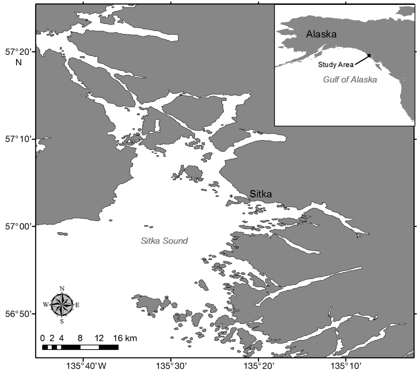
Figure 1. Map of Sitka Sound from Starr et al. 2011.
One of the many islands within the sound is Japonski Island, home to the University of Alaska Southeast (UAS) Sitka Campus Whale Lab, led by Dr. Lauren Wild and Dr. Ellen Chenoweth. The Whale Lab, previously led by Professor emeritus Jan Straley, has been monitoring whales for over 40 years. Through a myriad of data collection methods including photographic-identification (photo-ID), tissue samples, acoustic recordings, and accelerometry tags, the lab investigates whale diets, genetics, population dynamics, human-cetacean interaction, movement, and foraging ecology. With such rich datasets and, more importantly, deep ties to the community, the Whale Lab has long been a leader in understanding the whales of Sitka Sound.
Since around 2019, the Whale Lab has noted a marked increase in gray whales coming into the sound to take advantage of the pulsed resource of the spring herring spawn (from fewer than 20 individuals prior to 2019, to more than 150 individuals since 2019). Gray whales have been opportunistically monitored by the Whale Lab since the 1990s. To get a better understanding of the dynamic use of Sitka sound by these whales, the Whale Lab initiated a dedicated research program. Through collaboration with the Whale Lab, we in the GEMM Lab hope to learn more about the Sitka gray whales and the health and ecology of gray whales along the Oregon coast through comparative studies. But first, let’s get acquainted with the herring spawn!
The Herring Spawn
Pacific herring (Tlingit: Yaaw) are small schooling forage fish that spend most of their lives offshore, moving inshore each spring to spawn (NOAA Fisheries). However, Sitka Sound is unique because some herring overwinter locally in deeper trenches on both the southeast and western sides of the sound, helping to sustain a productive ecosystem year-round. As they approach the spawning season, the herring stay deeper in the canyons, waiting for sea surface temperatures to reach a threshold suitable for spawning (Harley et al. 2024). Once conditions are right, they move farther up in the water column and further into Sitka Sound. This draws in predators like humpback whales that forage on the adult herring using behaviors like bubble-net feeding.
Humpbacks aren’t the only ones targeting the adult herring. In Southeast Alaska, herring are harvested by humans in the spring for their roe using purse seines. Fishery openings are timed based on abundance, distribution, size, population structure, and past trends. The goal of the Sitka sac roe fishery is to sustainably harvest adults with the highest quality roe, meaning that specific fishing areas will open when pre-spawning fish are abundant and areas will close or be reduced when spawning begins (Dupuis et al. 2026). Sitka supports a robust herring fishery and is one of the last remaining sac roe fisheries in the state of Alaska (ADFG Herring Timeline).
Herring are broadcast spawners and synchronize the timing of the eggs (roe) release and the sperm (milt). The release of milt is what causes the water to turn that characteristic light turquoise color. Spawning occurs continuously for roughly two weeks, though timing varies by year. The eggs are incredibly adhesive, sticking to each other, kelp, seagrass, rocks, and even settling onto mats over the benthos.
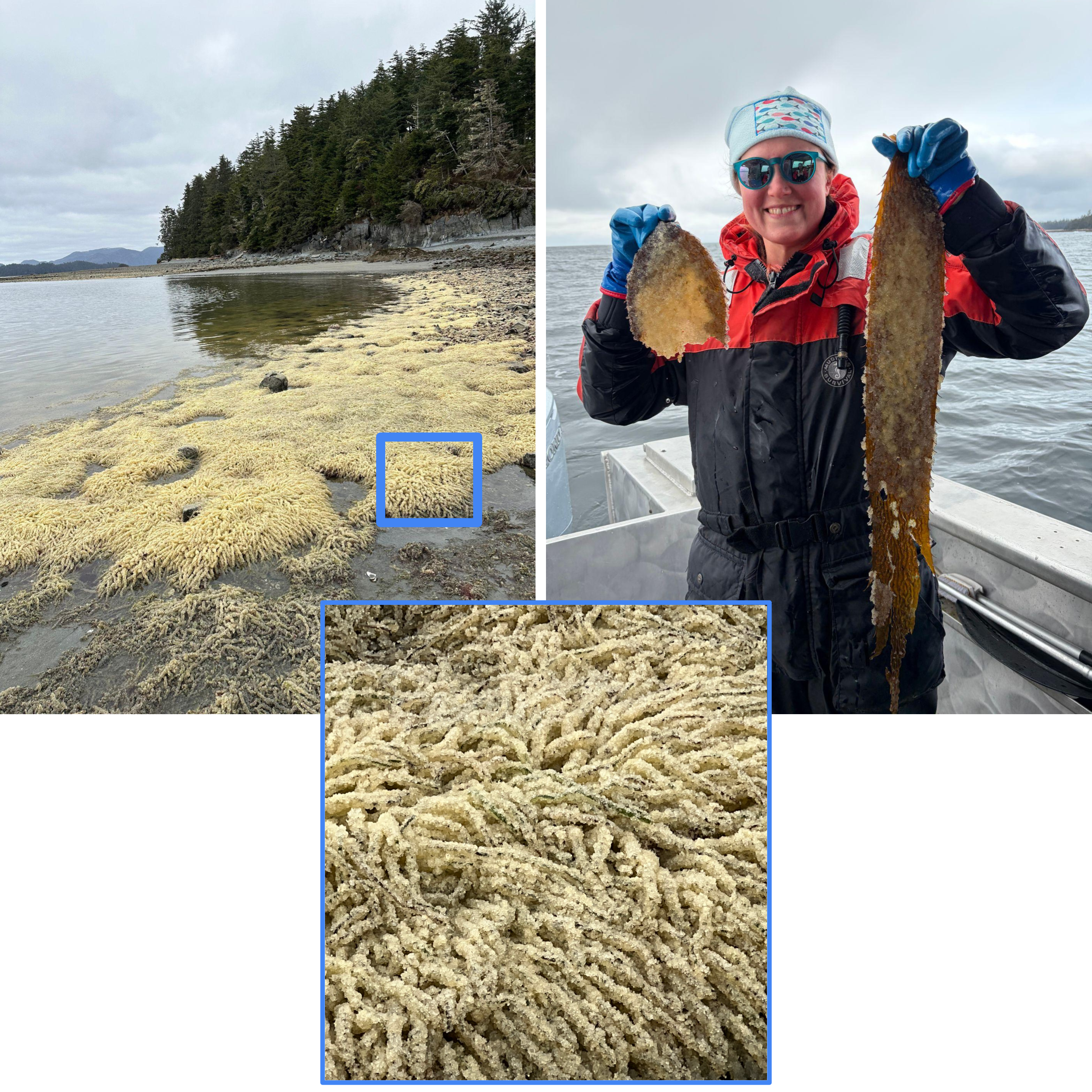
Figure 2. (Left) Eelgrass beds at low tide with herring eggs, (Center) closer image showing more detail of herring eggs attached to eelgrass and (Right) Willa Johnson holding kelp blades with attached herring eggs | Photo Credit: Willa Johnson (left, center) & Dr. Lauren Wild (right)
The huge quantity of eggs settles to the bottom and form mats that provide a rich nutrient source for many organisms. Another important harvest occurs at this point in the spawn: the cultural, traditional, and subsistence harvest of the eggs. Tlingit people have harvested herring eggs as an important food source and cultural resource for over 10,000 years. One of the Tlinigt clans, Kiks.ádi, is even named for them, with the women of the clan being called the herring ladies. The Tlingit and Haida method of gathering herring eggs involves placing hemlock boughs in the water, allowing herring to spawn on the branches, which are then collected (Thornton 2019; Theriault Boots 2026). Any eggs or branches not needed are returned to the ocean to contribute back to the ecosystem, so no food is wasted.
A single fertilized herring egg takes about two weeks to develop and hatch. After hatching, the herring larvae remain in the nearshore waters for a couple of weeks to months, though ocean conditions may advect some out of the sound. Due to the sheer size of the broadcast spawning event, there are inevitably eggs that go unfertilized or don’t survive to hatching. As a result, multiple developmental stages (hatched larvae, live developing eggs, and dead eggs) can coexist in the same area. These stages may differ in their distribution, caloric value, and availability, creating a complex and dynamic resource landscape for predators.
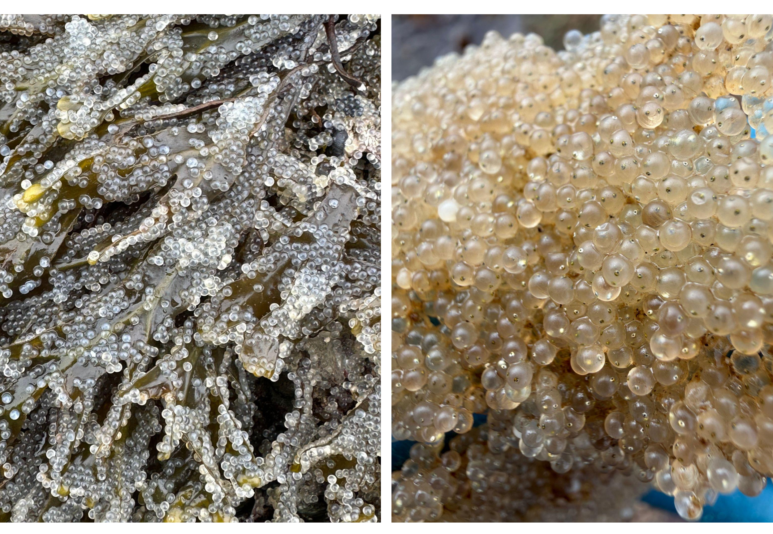
Figure 3. (Left) undeveloped herring eggs attached to Fucus distichus and (Right) herring eggs that have developed eyes or “eyed out” | Photo Credit: Willa Johnson (left) & Dr. Lauren Wild (right)
Bringing in the Whales
Now that we have a sense of the significance and timing of the herring spawn in Sitka Sound, let’s bring in the gray whales! Unlike humpback whales, which target adult herring, gray whales are sticking around for the herring spawn itself. Over the past seven years, the Whale Lab has noted an increased presence of gray whales within the sound. One of their hypotheses for this increase is that a spatial shift of the herring spawn closer to the mouth of the sound has allowed northbound migrating gray whales to detect and track this resource. Another draw may be a lack of predictability and reliability in other food sources for gray whales in their more traditional feeding grounds.
This unique ecological system is the source of endless questions: How many herring eggs are the gray whales consuming? Do whales that forage on this herring spawn gain an energetic advantage at the beginning of the foraging season? Where do these whales go after leaving Sitka Sound? Do PCFG whales incorporate this foraging opportunity into their broader foraging strategies? What impact is this increased feeding aggregation having on the herring biomass in Sitka Sound? Is this new prey resource supporting gray whale population resilience to declining prey availability in the Arctic? These questions span from local to basin-wide scales, and from individual gray whale to population levels. Collaborations between the Whale Lab and the GEMM Lab allow us to address different facets of these questions more effectively, with broader impacts for local communities, gray whale populations, and the broader scientific community.
Having a Field Day!
How are we beginning to answer these questions? Dr. Wild and Dr. Chenoweth lead field seasons to capture gray whale data using photo-ID, biopsies, Go-Pro imagery, and herring roe sampling, and net-tows. I was fortunate enough to join for a week of the Whale Lab’s field season and expand their efforts by incorporating drone imagery! With drone data, we can quantify body condition and capture fine-scale behavioral patterns, particularly the tactics whales use to forage on herring roe.
The morning after I arrived, we were on the water by 9:00, heading across the sound to Fred’s Creek. I met Dr. Wild’s incredible field team including Stacey Golden – a teacher in Sitka, Kaleigh Shroeder – a fish hatchery technician, Willa Johnson – a student at the University of Alaska Fairbanks (who I would meet the next day), and Dr. Wild herself. Having flown into Sitka in the dark, I was struck with the scenery surrounding us on our trip out.
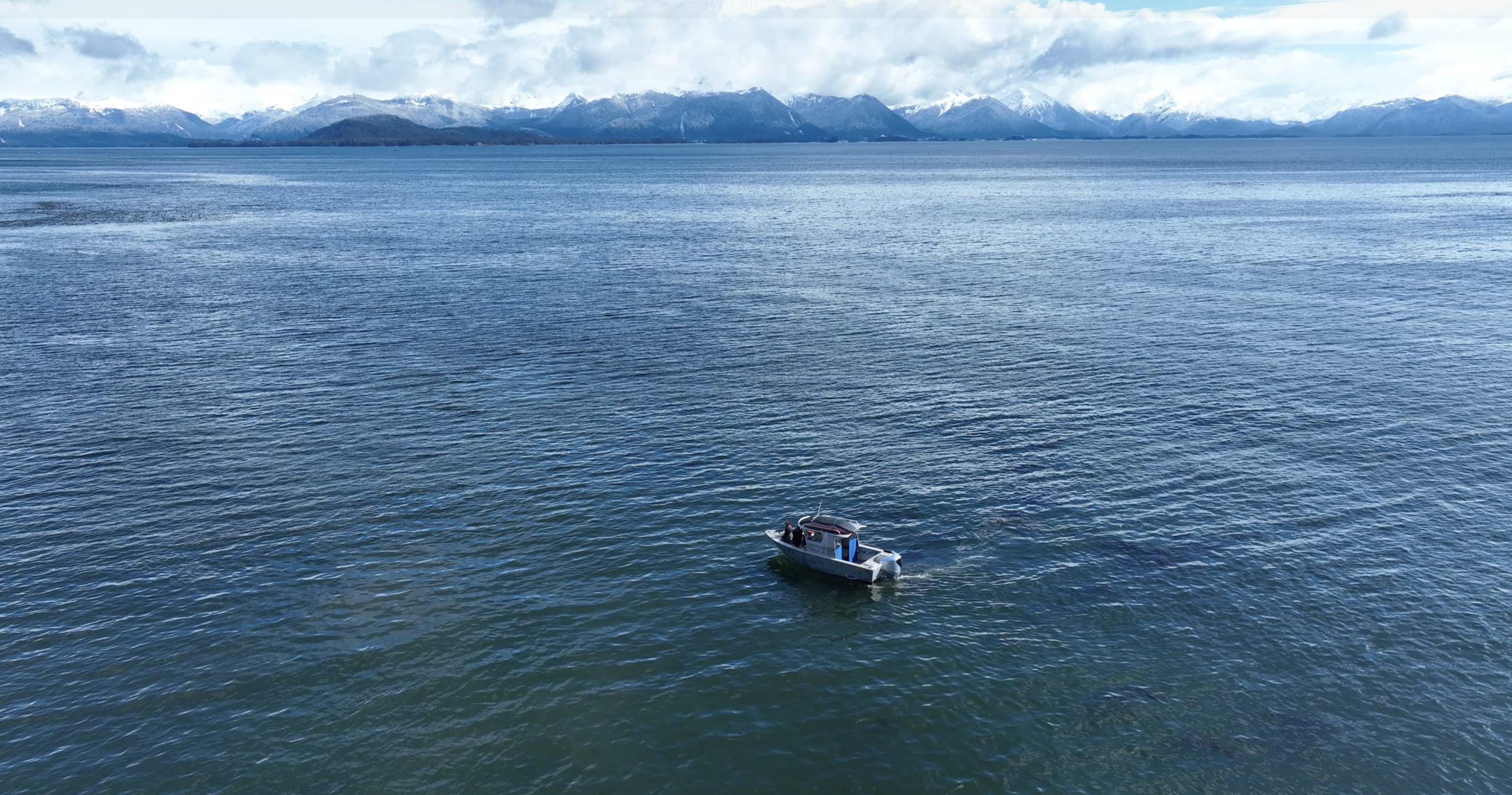
Figure 4. Dr. Wild’s research vessel facing east towards the mountains.
And it wasn’t just the mountains that were striking. As we approached the shoreline along the base of Mount Edgecumbe, I couldn’t believe my eyes when I started counting the number of blows that I was seeing. In just three hours with the Whale Lab on the first day, the best estimate of the number of whales was 28… this was whale soup! Once we reached a group of whales near the shore, we got to work. Stacey captured photo-ID pictures of each whale, Kaleigh recorded meticulous data and prepared for biopsy opportunities, I launched the drone, and Dr. Wild expertly maneuvered the boat among the whales and kelp beds. From a birds-eye view, I was able to see these groups of whales headstanding, aggregating in dense foraging groups, and even logging at the surface.Figure 4. Dr. Wild’s research vessel facing east towards the mountains.
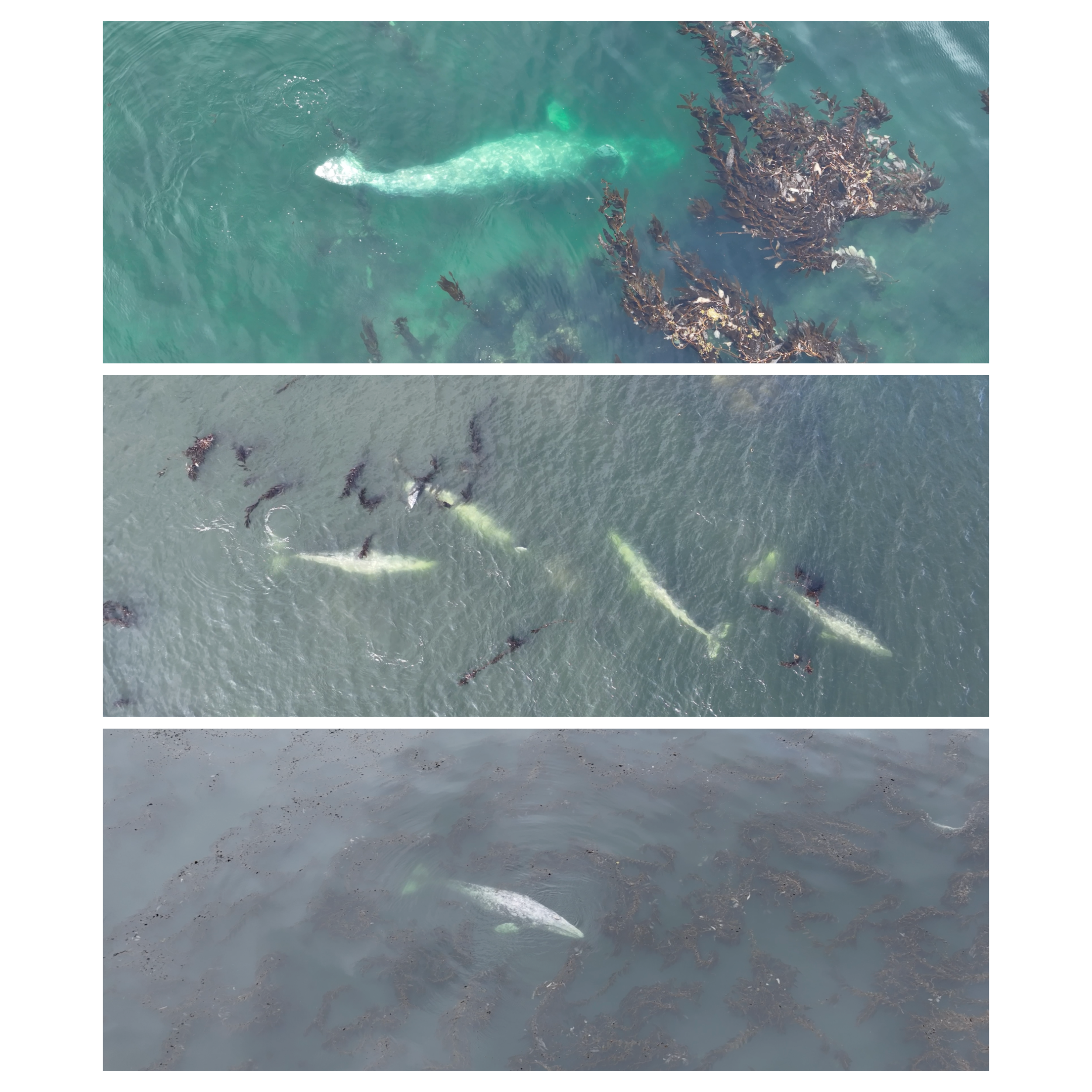
Figure 5. (Top) whale exhibiting a headstand next to a kelp bed with attached herring eggs, (Middle) 4 whales foraging and traveling close together, and (Bottom) a whale logging amidst a kelp bed.
The aerial view also revealed the environmental context of these behaviors. Patches of herring roe were clearly visible, clinging to kelp in the water. It wasn’t until later that afternoon, when the fieldwork adrenaline settled and I started reviewing the drone footage, that I began to fully appreciate the complexity of what we had observed.
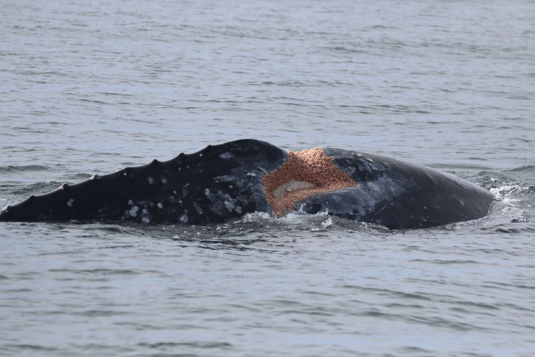
On the second day, I was able to capture one of the fascinating behaviors Dr. Wild had described: gray whales actively scraping herring eggs off kelp. While a majority of the gray whales were headstanding and foraging on the roe associated with the benthos, there were other whales pushing through kelp beds, tearing at the blades to access the eggs attached. This behavior may have broader implications, particularly for kelp-associated communities and the zooplankton species that rely on kelp as refugia later in the season – one of the many fascinating open questions about this elaborate system. That second day was also our largest survey effort of that week, with a best estimate of 154 gray whales observed along our transect!
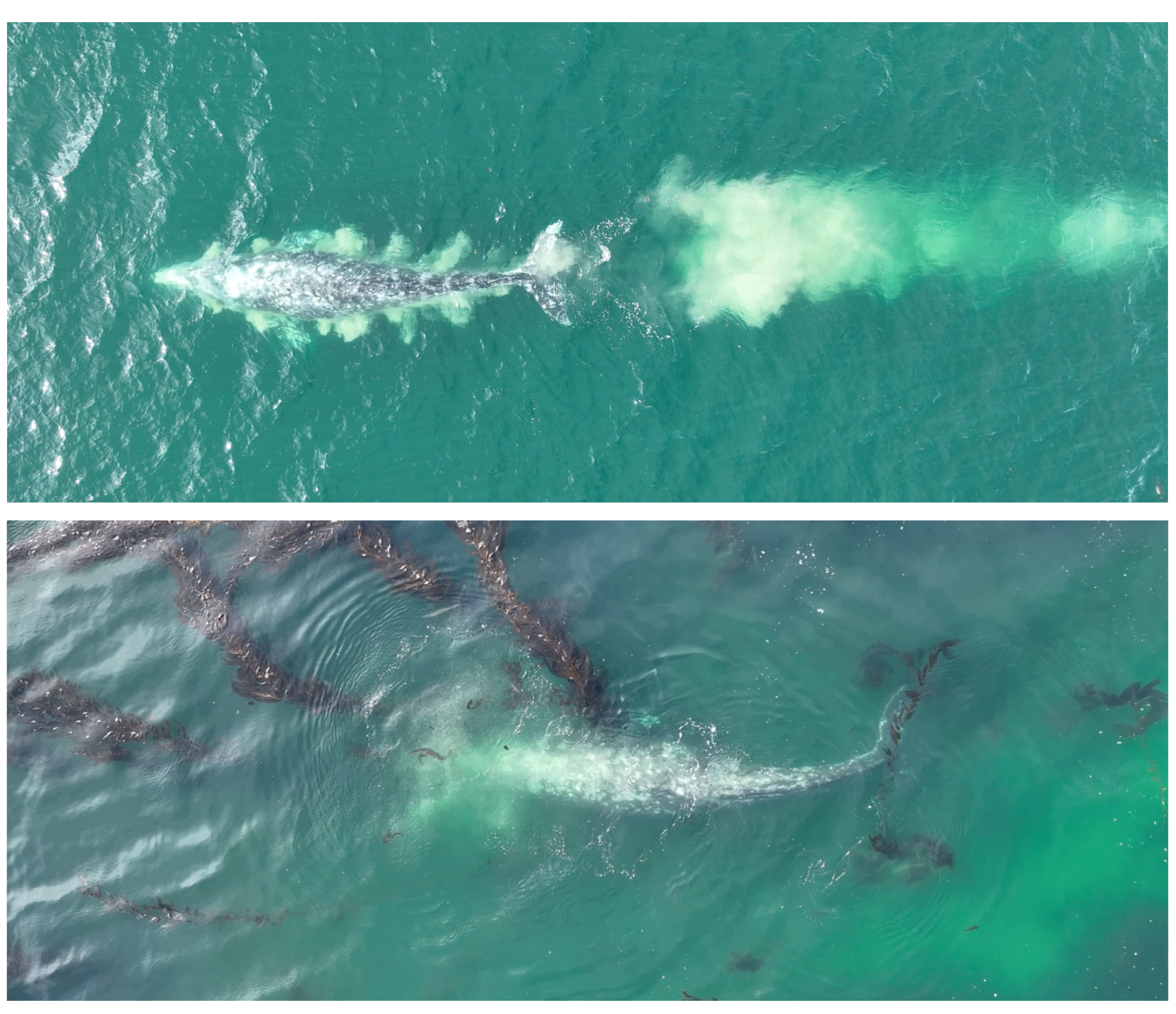
Figure 6. (Top) Gray whale filtering sediment after foraging in the benthos and (Bottom) gray whale stripping kelp to acquire attached herring spawn.
After returning to shore, I attended a Sitka Natural History Seminar by Matt Goff, a local naturalist who has dedicated himself to documenting and learning about Sitkan ecology. His talk, “Getting to Know our Neighbors”, highlighted a few of the over 3,000 species that he has documented on iNaturalist within the Sitka region. He also maintains a blog that documents his observations and a radio show where he hosts conversations with community members and scientists, including an October 4th, 2024 show where he interviews Dr. Wild about the gray whales.
The following day would end up being the last opportunity to fly the drone. By then, the coordination of the drone operations into the Whale Lab’s fieldwork had become seamless – calling out notes and timestamps, aligning observations, and integrating multiple data streams real time. Although the rain grounded the drone on the last day, we were still able to get out on the sound and collect photo-ID data and tissue samples with Dr. Chenoweth as well as Scott Simmons – a UAS dive instructor. As we drove back into the harbor I was trying to savor every second of being on the water in this incredible place, with these incredible people.
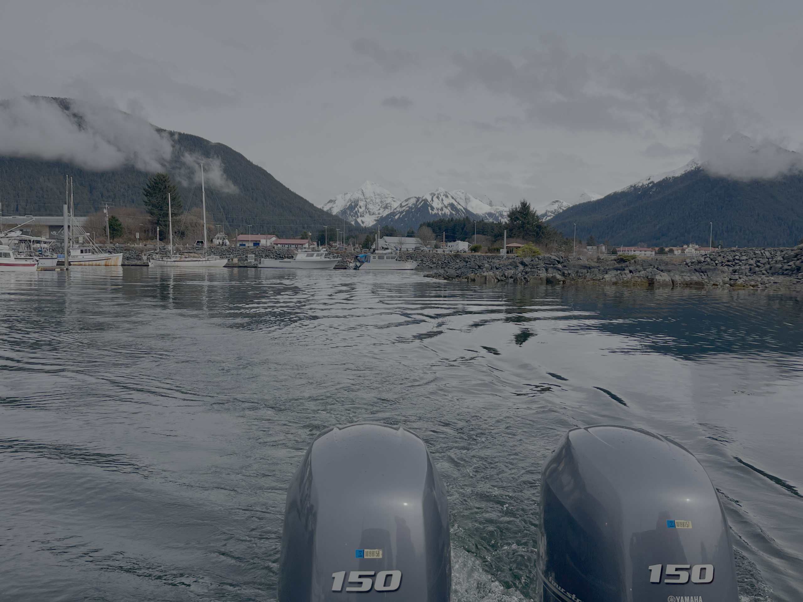
Figure 7. Coming into harbor with the Three Sisters mountains in the background.
Having come into an established, long-term gray whale study in Newport, Oregon (GRANITE), and then being able to experience another established, long-term gray whale study in Sitka, Alaska (Whale Lab) is a rare privilege. I am so grateful to Dr. Wild and Dr. Chenoweth for welcoming me into their homes, labs, and community. Experiencing these different ecosystems and being a part of a collaboration between two major gray whale research programs is deeply inspiring, especially at such an exciting time in gray whale research.
What the Future Holds
Looking ahead, the strength of this collaboration lies not just in the questions we are asking now, but in how adaptable this system is to the rapidly changing conditions gray whales are experiencing. As gray whales continue to navigate population-level fluctuations, understanding how localized foraging opportunities like the Sitka herring spawn fit into broader energetic and health dynamics is becoming increasingly important. Moreover, understanding the effects of the increasing number of gray whales in regions that they haven’t previously used intensively is critical for addressing questions about localized ecological impacts and community interactions. By pairing the Whale Lab’s fine-scale, system-specific work on bioenergetics and consumption with the GEMM Lab’s broader, range-wide perspective on gray whale health and ecology, we can begin to piece together how these whales are responding to shifting ecosystems. These insights are only possible through sustained monitoring and strong, reciprocal collaborations, not just between research groups, but with the communities who live alongside and are deeply connected to these whales. As generalist foragers operating across diverse and dynamic habitats, gray whales challenge us to think across scales, disciplines, and perspectives, making this continued collaborative effort more important than ever.
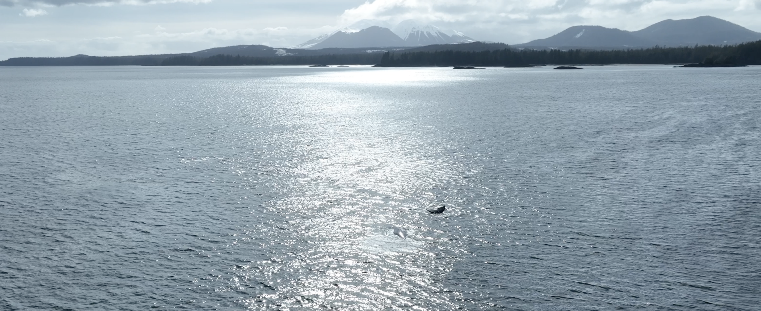
Figure 8. Photo of two whales surfacing in front of Mount Edgecumbe
Acknowledgements
I would like to first and foremost acknowledge the Tlingit people, who have stewarded the lands and waters around Sitka for over 10,000 years, and on whose homelands we are guests. Immense thank you to Dr. Lauren Wild and Dr. Ellen Chenoweth for hosting me and additional thanks to Dr. Wild for proofreading the first draft of this blog.
References
ADFG Herring Timeline, n.d. TIMELINE OF COMMERCIAL HERRING FISHERIES IN SOUTHEAST ALASKA.
Boots, M.T., n.d. In Sitka, spring herring spawn yields a subsistence treasure to be shared [WWW Document]. Anchorage Daily News. URL https://www.adn.com/alaska-news/rural-alaska/2026/04/18/in-sitka-spring-herring-spawn-yields-a-subsistence-treasure-to-be-shared/ (accessed 5.1.26).
Dupuis, A., Forbes, S., Meredith, B., n.d. 2026 Southeast Alaska herring sac roe fishery management plan.
Heintz, R., Moran, J., Vollenweider, J., Straley, J., Boswell, K., Rice, J., 2010. Humpback Whale Predation and the Case for Top-Down Control of Local Herring Populations in the Gulf of Alaska.
Liddle, J.B., 2015. Population dynamics of Pacific herring and humpback whales, Sitka Sound, Alaska 1981-2011 (Ph.D.). ProQuest Dissertations and Theses. University of Alaska Fairbanks, United States — Alaska.
NOAA, 2023. Pacific Herring | NOAA Fisheries [WWW Document]. NOAA. URL https://www.fisheries.noaa.gov/species/pacific-herring (accessed 5.1.26).
Starr, R., O’Connell, V., Ralston, S., 2011. Movements of lingcod (Ophiodon elongatus) in southeast Alaska: Potential for increased conservation and yield from marine reserves. Canadian Journal of Fisheries and Aquatic Sciences 61, 1083–1094. https://doi.org/10.1139/f04-054
Thornton, 2019. New study shows social, cultural, ecological benefits of herring subsistence economy are at risk [WWW Document]. University of Alaska Southeast. URL https://uas.alaska.edu/about/press-releases/2019/191122-herring-roe.html (accessed 5.1.26).
Wild, L.A., Riley, H.E., Pearson, H.C., Gabriele, C.M., Neilson, J.L., Szabo, A., Moran, J., Straley, J.M., DeLand, S., 2023. Biologically Important Areas II for cetaceans within U.S. and adjacent waters – Gulf of Alaska Region. Front. Mar. Sci. 10. https://doi.org/10.3389/fmars.2023.1134085