oceanography – Geospatial Ecology of Marine Megafauna Laboratory

The Dark Side of Upwelling: It’s getting harder and harder to breathe off the Oregon coast

By Rachel Kaplan, PhD candidate, Oregon State University College of Earth, Ocean, and Atmospheric Sciences and Department of Fisheries, Wildlife, and Conservation Sciences, Geospatial Ecology of Marine Megafauna Lab

The depths of the productive coastal Oregon ecosystem have long held a mystery – an increasing paucity in the concentration of dissolved oxygen at depth. When dissolved oxygen concentrations dips low enough, the condition “hypoxia” can alter biogeochemical cycling in the ocean environment and threaten marine life. Essentially, organisms can’t get enough oxygen from the water, forcing them to try to escape to more favorable waters, stay and change their behavior, or suffer the consequences and potentially suffocate.

Recent work has illuminated the cause of this mysterious rise in hypoxic waters: an increase in the wind-driven oceanographic process of upwelling (Barth et al., 2024). The seasonal upwelling of cold, nutrient-rich waters underlies the incredible productivity of the Oregon coast, but its dark twin is hypoxia: when organic material in the upper layer of the water column sinks, microbial respiration processes consume dissolved oxygen in the surrounding water. In addition, the deep waters brought to the surface by upwelling are depleted in oxygen compared to the aerated surface waters. These effects combine to form an oxygen-poor water layer over the continental shelf, which typically lasts from May until October in the Northern California Current (NCC) region. The spatial extent of this layer is highly variable – hypoxic bottom waters cover 10% of the shelf in some years and up to 62% in others, presenting challenging conditions for life occupying the Oregon shelf (Peterson et al., 2013).

Figure 1. An article in The Oregonian from 2004 documents research on a hypoxia-driven “dead zone” off the Oregon coast.

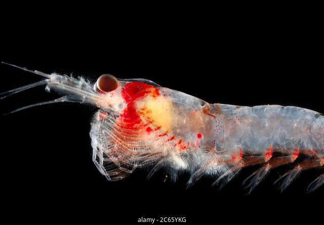
While effects of hypoxia on benthic communities and some fish species are well-documented, is unclear how increasing levels of hypoxia off Oregon may impact highly mobile, migratory organisms like whales. A primary pathway is likely through their prey – particularly species that occupy hypoxic regions and depths, like the zooplankton krill. Over the continental shelf and slope, which are important krill habitat, seasonally hypoxic waters tend to extend from about 150 meters depth to the bottom. The vertical center of krill distribution in the NCC region is around 170 meters depth, suggesting that these animals encounter hypoxic conditions regularly.

Interestingly, the two main krill species off the Oregon coast, Euphausia pacifica and Thysanoessa spinifera, use different strategies to deal with hypoxic conditions. Thysanoessa spinifera krill decrease their oxygen consumption rate to better tolerate ambient hypoxia, a behavioral modification strategy called “oxyconformity”. Euphausia pacifica, on the other hand, use “oxyregulation” to maintain the same, quite high, oxygen utilization rate regardless of ambient levels – which may indicate that this species will be less able to tolerate increasingly hypoxic waters (Tremblay et al., 2020).

Figure 2. This figure from Barth et al. 2024 maps the concentration of dissolved oxygen (uM/kg; cooler colors indicate less dissolved oxygen) to show an increase in hypoxic conditions over the continental shelf and slope (green and blue colors) across seven decades in the NCC region.

Over long time scales, such environmental pressures shape species physiology, life history, and evolution. The krill species Euphausia mucronate is endemic to the Humboldt Current System off the coast of South America, which includes a region of year-round upwelling and a persistent Oxygen Minimum Zone (OMZ). Fascinatingly, Humboldt krill can live in the core of the OMZ, using metabolic adaptations that even let them survive in anoxic conditions (i.e., no oxygen in the water). Humboldt krill abundances actually increase with shallower OMZ depths and lower levels of dissolved oxygen, pointing to the huge success of this species in evolving to thrive in conditions that challenge other local krill species (Díaz-Astudillo et al., 2022).

Back home in the NCC region, will Euphausia pacifica and Thysanoessa spinifera be pressured to adapt to continually increasing levels of hypoxia? If so, will they be able to adapt? One of krill’s many superpowers is an ability to tolerate a wide range of environmental conditions, including the dramatic gradients in temperature, water density, and dissolved oxygen that they encounter during their daily vertical migrations through the water column. Both species have strategies to deal with hypoxic conditions, and this capacity has allowed them to thrive in the active upwelling region that is the NCC. Now, the question is whether increasingly hypoxic waters will eventually force a threshold that compromises the capacity of krill to adapt – and then, what will happen to these species, and the foragers dependent on them?

References

Barth, J. A., Pierce, S. D., Carter, B. R., Chan, F., Erofeev, A. Y., Fisher, J. L., Feely, R. A., Jacobson, K. C., Keller, A. A., Morgan, C. A., Pohl, J. E., Rasmuson, L. K., & Simon, V. (2024). Widespread and increasing near-bottom hypoxia in the coastal ocean off the United States Pacific Northwest. Scientific Reports, 14(1), 3798. https://doi.org/10.1038/s41598-024-54476-0

Díaz-Astudillo, M., Riquelme-Bugueño, R., Bernard, K. S., Saldías, G. S., Rivera, R., & Letelier, J. (2022). Disentangling species-specific krill responses to local oceanography and predator’s biomass: The case of the Humboldt krill and the Peruvian anchovy. Frontiers in Marine Science, 9, 979984. https://doi.org/10.3389/fmars.2022.979984

Peterson, J. O., Morgan, C. A., Peterson, W. T., & Lorenzo, E. D. (2013). Seasonal and interannual variation in the extent of hypoxia in the northern California Current from 1998–2012. Limnology and Oceanography, 58(6), 2279–2292. https://doi.org/10.4319/lo.2013.58.6.2279

Tremblay, N., Hünerlage, K., & Werner, T. (2020). Hypoxia Tolerance of 10 Euphausiid Species in Relation to Vertical Temperature and Oxygen Gradients. Frontiers in Physiology, 11, 248. https://doi.org/10.3389/fphys.2020.00248

Oceanographic Alchemy: How Winds Become Whale Food in Oregon

By Rachel Kaplan, PhD student, Oregon State University College of Earth, Ocean, and Atmospheric Sciences and Department of Fisheries, Wildlife, and Conservation Sciences, Geospatial Ecology of Marine Megafauna Lab

Here in the GEMM lab, we love the Oregon coast for its amazing animals – the whales we all study, the seabirds we can sometimes spot from the lab, and the critters that come up in net tows when we’re out on the water. Oregonians owe the amazing biological productivity of the Oregon coast to the underlying atmospheric and oceanographic processes, which make our local Northern California Current (NCC) ecosystem one of the most productive places on earth.

While the topographical bumps of the Oregon coastline and vagaries of coastal weather do have a big impact on the physical and biological processes off the coast, the dominant forces shaping the NCC are large-scale, atmospheric heavy hitters. As the northeasterly trade winds blow across the globe, they set up the clockwise-rotating North Pacific Subtropical Gyre, a major feature covering about 20 million square kilometers of the Pacific Ocean. The equatorward-flowing part of the gyre is the California Current. It comprises an Eastern Boundary Upwelling Ecosystem, one of four such global systems that, while occupying only 1% of the global ocean, are responsible for a whopping 11% of its total primary productivity, and 17% of global fish catch.

*Figure 1.* Important features of the California Current System (Checkley and Barth, 2009).

At its core, this incredible ocean productivity is due to atmospheric pressure gradients. Every spring, an atmospheric system called the North Pacific High strengthens, loosening the hold of the stormy Aleutian Low. As a result, the winds begin to blow from the north, pushing the surface water in the NCC with them towards the equator.

This water is subject to the Coriolis effect – an inertial force that acts upon objects moving across a rotating frame of reference, and the same force that airplane pilots must account for in their flight trajectories. As friction transmits the stress of wind acting upon the ocean’s surface downward through the water column, the Coriolis effect deflects deeper layers of water successively further to the right, before the original wind stress finally peters out due to frictional losses.

This process creates an oceanographic feature called an Ekman spiral, and its net effect in the NCC is the offshore transport of surface water. Deep water flows up to replace it, bringing along nutrients that feed the photosynthesizers at the base of the food web. Upwelling ecosystems like the NCC tend to be dominated by food webs full of large organisms, in which energy flows from single-celled phytoplankton like diatoms, to grazers like copepods and krill, to predators like fish, seabirds, and our favorite, whales. These bountiful food webs keep us busy: GEMM Lab research has explored how upwelling dynamics impact gray whale prey off the Oregon coast, as well as parallel questions far from home about blue whale prey in New Zealand.

*Figure 2. The Coriolis effect creates an oceanographic feature called an Ekman Spiral, resulting in water transport perpendicular to the wind direction (Source:* *NOAA*).

Although the process of upwelling lies at the heart of the productive NCC ecosystem, it isn’t enough for it to simply happen – timing matters, too. The seasonality of ecological events, or phenology, can have dramatic consequences for the food web, and individual populations in it. When upwelling is initiated as normal by the “spring transition”, the delivery of freshly upwelled nutrients activates the food web, with reverberations all the way from phytoplankton to predators. When the spring transition is late, however, the surface ocean is warm, nutrients are depleted, primary productivity is low, and the life cycles and abundances of some species can change dramatically. In 2005, for example, the spring transition was delayed by a month, resulting in declines and spatial redistributions of the taxa typically found in the NCC, including hake, rockfish, albacore tuna, and squid. The Cassin’s auklet, which feeds on plankton, suffered its worst year on record, including reproductive failure that may have resulted from a lack of food.

Upwelling is alchemical in its power to transform, modulating physical and atmospheric processes and turning them into ecosystem gold – or trouble. As oceanographers and Oregonians alike wonder how climate change may reshape our coast, changes to upwelling will likely play a big role in determining the outcome. Some expect that upwelling-favorable winds will become more prevalent, potentially increasing primary productivity. Others suspect that the timing of upwelling will shift, and ecological mismatches like those that occurred in 2005 will be increasingly detrimental to the NCC ecosystem. Whatever the outcome, upwelling is inherent to the character of the Oregon coast, and will help shape its future.

*Figure 3.* The GEMM Lab is grateful that the biological productivity generated by upwelling draws humpback whales like this one to the Oregon coast! (photo: Dawn Barlow)

References

Chavez, Francisco & Messié, Monique. (2009). A comparison of Eastern Boundary Upwelling Ecosystems. Progress In Oceanography. 83. 80-96. 10.1016/j.pocean.2009.07.032.

Chavez, F P., and J R Toggweiler, 1995: Physical estimates of global new production: The upwelling contribution. In Dahlem Workshop on Upwelling in the Ocean: Modern Processes and Ancient Records, Chichester, UK, John Wiley & Sons, 313-320.

Checkley, David & Barth, John. (2009). Patterns and processes in the California Current System. Progress In Oceanography. 83. 49-64. 10.1016/j.pocean.2009.07.028.

El Niño de Navidad: What is atmospheric Santa Claus bringing to Oregon krill and whales?

Early June marked the onset of El Niño conditions in the Pacific Ocean , which have been strengthening through the fall and winter. For Oregonians, this climate event means unseasonably warm December days, less snow and overall precipitation (it’s sunny as I write this!), and the potential for increased wildfires and marine heatwaves next summer.

This phenomenon occurs about every two to seven years as part of the El Niño Southern Oscillation (ENSO), a cyclical rotation of atmospheric and oceanic conditions in the Pacific Ocean that is initiated by departures from and returns to “normal conditions” at the equator. Typically, the trade winds blow warm water west along the equator, and El Niño occurs when these winds weaken or reverse. As a result, the upwelling of cold water at the equator ceases, and warm water flows towards the west coast of the Americas, rather than its typical pathway towards Asia. When the trade winds resume their normal direction, usually after months or a year, the system returns to “normal” conditions – or, it can enter the cool La Niña part of the cycle, in which the trade winds are stronger than normal. “El Niño de Navidad” was named by South American fisherman in the 1600s because this event tends to peak in December – and El Niño is clearly going to be a guest for Christmas this year.

*Figure 1.* Maps of sea surface temperature anomalies show Pacific Ocean conditions during a strong La Niña (top) and El Niño (bottom). Source: NOAA climate.gov

These events at the equator trigger changes in global atmospheric circulation patterns, and they can shape weather around the world. Teleconnection, the coherence between meteorological and environmental phenomena occurring far apart, is to me one of the most incredible things about the natural world. This coherence means that the biological community off the Oregon coast is strongly impacted by events initiated at the equator, with consequences that we don’t yet fully understand.

The effects of El Niño are diverse – floods in some places, droughts in others – and their onset can mean wildly different things for Oregon, Peru, Alaska, and beyond. As we tap our fingers waiting to be able to ski and snowboard in Oregon, what does our current El Niño event mean for the life in the waters off our coast?

*Figure 2.* Anomalous conditions at the equator qualified as an El Niño event in June 2023.

ENSO plays a big role in the variability in our local Northern California Current (NCC) system, and the outcomes of these events can differ based on the strength and how the signal propagates through the ocean and atmosphere (Checkley & Barth, 2009). Large-scale “coastal-trapped” waves flowing alongshore can bring the warm water signal of an El Niño to our ocean backyard in a matter of weeks. One of the first impacts is a deepening of the thermocline, the upper ocean’s steep gradient in temperature, which changes the cycling of important nutrients in the surface ocean. This can result in a decrease in upwelling and primary productivity that sends ramifications through the food web, including consequences for grazers and predators like zooplankton, marine mammals, and seabirds (Checkley & Barth, 2009).

In addition to these ecosystem effects that result from local changes, the ocean community can also receive new visitors from afar, and see others flee . For krill, the shrimp-like whale prey that I spend a lot of my time thinking about, community composition can change as subtropical species typically found off southern and Baja California are displaced by horizontal ocean flow, or as resident species head north (Lilly & Ohman, 2021).

*Figure 3*. This *Euphausia gibboides* krill is typically found in offshore subtropical habitats but moves north and inshore during El Niño events, and tends to persist awhile in these new environments, impacting the local zooplankton community. Source: Solvn Zankl

The two main krill species that occur in the NCC, Euphausia pacifica and Thysanoessa spinifera, favor the cool, coastal waters typical off the coast of Oregon. During El Niño events, E. pacifica tends to contract its distribution inshore in order to continue occupying these conditions, increasing its spatial overlap with T. spinifera (Lilly & Ohman, 2021). In addition, both tend to shift their populations north, toward cooler, upwelling waters (Lilly & Ohman, 2021).

These krill species are a favored prey of rorqual whales, and the coast of Oregon is an important foraging ground for humpback, blue, and fin whales. Predators tend to follow their prey, and shifting distributions of these krill species may cause whales to move, too. During the 2014-2015 “Blob” event in the Pacific Ocean, a marine heatwave was exacerbated by El Niño conditions. Humpback whales in central California shifted their distributions inshore in response to sparse offshore krill, increasing their overlap with fishing gear and leading to an increase in entanglement events (Santora et al., 2020). Further north, these conditions even led humpback whales to forage in the Columbia River!

Figure 4. In September 2015, El Niño conditions led humpback whales to follow their prey and forage in the Columbia River.

As El Niño events compound with the impacts of global climate change, we can expect these distributional shifts – and perhaps surprises – to continue. By the year 2100, the west coast habitat of both T. spinifera and E. pacifica will likely be constrained due to ocean warming – and when El Niños occur, this habitat will decrease even further (Lilly & Ohman, 2021). As a result, the abundances of both species are expected to decrease during El Niño events, beyond what is seen today (Lilly & Ohman, 2021). This decline in prey availability will likely present a problem for future foraging whales, which may already be facing increased environmental challenges.

Understanding connections is inherent to the field of ecology, and although these environmental dependencies are part of what makes life so vulnerable, they can also be a source of resilience. Although humans have known about ENSO for over 400 years, the complex interplay between nature, anthropogenic systems, and climate change means that we are still learning the full implications of these events. Just as waiting for Santa Claus always keeps kids guessing, the dynamic ocean keeps surprising us, too.

References

Checkley, D. M., & Barth, J. A. (2009). Patterns and processes in the California Current System. Progress in Oceanography, 83(1–4), 49–64. https://doi.org/10.1016/j.pocean.2009.07.028

Lilly, L. E., & Ohman, M. D. (2021). Euphausiid spatial displacements and habitat shifts in the southern California Current System in response to El Niño variability. Progress in Oceanography, 193, 102544. https://doi.org/10.1016/j.pocean.2021.102544

Santora, J. A., Mantua, N. J., Schroeder, I. D., Field, J. C., Hazen, E. L., Bograd, S. J., Sydeman, W. J., Wells, B. K., Calambokidis, J., Saez, L., Lawson, D., & Forney, K. A. (2020). Habitat compression and ecosystem shifts as potential links between marine heatwave and record whale entanglements. Nat Commun, 11(1), 536. https://doi.org/10.1038/s41467-019-14215-w

A Matter of Time: Adaptively Managing the Timescales of Ocean Change and Human Response

By Rachel Kaplan, PhD student, OSU College of Earth, Ocean and Atmospheric Sciences and Department of Fisheries, Wildlife, & Conservation Sciences, Geospatial Ecology of Marine Megafauna Lab

Ocean ecosystems are complex and dynamic, shaped by the interconnected physical and biogeochemical processes that operate across a variety of timescales. A trip on the “ocean conveyer belt”, which transports water from the North Atlantic across the global ocean and back in a process called thermohaline circulation, takes about a thousand years to complete. Phytoplankton blooms, which cycle nutrients through the surface ocean and feed marine animals, often occur at the crucial, food-poor moment of spring, and last for weeks or months. The entanglement of a whale in fishing gear, a major anthropogenic threat to ocean life that drives the GEMM Lab’s Project OPAL, can happen in seconds.

Compounding this complexity, even the timescales that research has clarified are changing. Many processes in the ocean are shifting – and often accelerating – due to global climate change. Images of melting sea ice, calving glaciers, and coastal erosion all exemplify our natural world’s rapid reorganization, and even discrete events can have dramatic repercussions and leave their mark for years. For example, a marine heatwave that occurred in 2014-2015 raised temperatures up to 2.5° C warmer than usual, redistributed species northward along the United States’ West Coast, spurred harmful algal blooms, and shut down fisheries. The toxic blooms also caused marine mammal strandings, domoic acid poisoning in California sea lions, and seabird mass death events (McCabe et al., 2016).

***Figure 1.*** *Figures like this Stommel diagram reveal the broad temporal and spatial scales over which ocean phenomena occur. Source: Sloyan et al., 2019*

As humans seek to manage ocean ecosystems and mitigate the effects of climate change, our political processes have their own time scales, interconnected cycles, and stochasticity, just like the ocean. At the federal level in the United States, the legislative process takes place over months to decades, sometimes punctuated by relatively quicker actions enacted through Executive Orders. In addition, just as plankton have their turnover times, so do governmental branches. Both the legislative branch and the executive branch change frequently, with new members of Congress coming in every two years, and the president and administration changing every four or eight years. Turnover in both of these branches may constitute a total regime shift, with new members seeking to redirect science policy efforts.

The friction between oceanic and political timescales has historically made crafting effective ocean conservation policy difficult. In recent years, the policy approach of “adaptive management” has sought to respond to the challenges at the tricky intersection of politics, climate change, and ocean ecosystems. The U.S. Department of the Interior’s Technical Guide to Adaptive Management highlights its capacity to deal with the uncertainty inherent to changing ecosystems, and its ability to accommodate progress made through research: “Adaptive management [is a decision process that] promotes flexible decision making that can be adjusted in the face of uncertainties as outcomes from management actions and other events become better understood. Careful monitoring of these outcomes both advances scientific understanding and helps adjust policies or operations as part of an iterative learning process” (Williams et al, 2009).

Over the last several years, adaptive management policy approaches have been key as resource managers along the West Coast have responded to the problem of whale entanglement in fishing gear. When the 2014-2015 marine heatwave event caused anomalously low krill abundance in the central California Current region, humpback whales used a tactic called “prey-switching”, and fed on inshore anchovy schools rather than offshore krill patches. The resulting habitat compression fueled an increase in humpback whale entanglement events in Dungeness crab fishing gear (Santora et al, 2020).

This sudden uptick in whale entanglements necessitated strategic management responses along the West Coast. In 2017, the California Dungeness Crab Fishing Gear Working Group developed the Risk Assessment and Mitigation Program (RAMP) to analyze real-time whale distribution and ocean condition data during the fishing season, and provide contemporaneous assessments of entanglement risk to the state’s Department of Fish and Wildlife. The Oregon Whale Entanglement Working Group (OWEWG) formed in 2017, tasked with developing options to reduce risk. Oregon Department of Fish and Wildlife (ODFW) has guided whale entanglement reduction efforts by identifying four areas of ongoing work: accountability, risk reduction, best management practices, and research – with regular, scheduled reviews of the regulations and opportunities to update and adjust them.

***Figure 2.*** *Entanglement in fishing gear can occur in seconds and may negatively impact whales for years. Source Scott Benson/NOAA*

The need for research to support the best possible policy is where the GEMM Lab comes in. ODFW has established partnerships with Oregon State University and Oregon Sea Grant in order to improve understanding of whale distributions along the coast that can inform management efforts. Being involved in this cooperative “iterative learning process” is exactly why I’m so glad to be part of Project OPAL. Initial results from this work have already shaped ODFW’s regulations, and the framework of adaptive management and assessment means that regulations can continue being updated as we learn more through our research.

Ecosystem management will always be complex, just like ecosystems themselves. Today, the pace at which the climate is changing causes many people concern and even despair (Bryndum-Buchholz, 2022). Building adaptive approaches into marine policymaking, like the ones in use off the West Coast, introduces a new timescale into the U.S. policy cycle – one more in line with the rapid changes that are occurring within our dynamic ocean.

References

Williams, B. L., Szaro, R. C., and Shapiro, C. D. 2009. Adaptive management: the U.S. Department of the Interior Technical Guide. Adaptive Management Working Group, v pp.

Bryndum-Buchholz, A. (2022). Keeping up hope as an early career climate-impact scientist. ICES Journal of Marine Science, 79(9), 2345–2350. https://doi.org/10.1093/icesjms/fsac180

McCabe, R. M., Hickey, B. M., Kudela, R. M., Lefebvre, K. A., Adams, N. G., Bill, B. D., Gulland, F. M., Thomson, R. E., Cochlan, W. P., & Trainer, V. L. (2016). An unprecedented coastwide toxic algal bloom linked to anomalous ocean conditions. Geophys Res Lett, 43(19), 10366–10376. https://doi.org/10.1002/2016GL070023

Santora, J. A., Sydeman, W. J., Schroeder, I. D., Wells, B. K., & Field, J. C. (2011). Mesoscale structure and oceanographic determinants of krill hotspots in the California Current: Implications for trophic transfer and conservation. Progress in Oceanography, 91(4), 397–409. https://doi.org/10.1016/j.pocean.2011.04.002

Sloyan, B. M., Wilkin, J., Hill, K. L., Chidichimo, M. P., Cronin, M. F., Johannessen, J. A., Karstensen, J., Krug, M., Lee, T., Oka, E., Palmer, M. D., Rabe, B., Speich, S., von Schuckmann, K., Weller, R. A., & Yu, W. (2019). Evolving the Physical Global Ocean Observing System for Research and Application Services Through International Coordination. Frontiers in Marine Science, 6, 449. https://doi.org/10.3389/fmars.2019.00449

Coming full circle

By Rachel Kaplan, PhD student, OSU College of Earth, Ocean, and Atmospheric Sciences and Department of Fisheries and Wildlife, Geospatial Ecology of Marine Megafauna Lab

Returning to a place you once lived always shows how much you and the world around you have changed, offering a new perspective on the time away and where you are now. I’m writing this from my old office at Bigelow Laboratory for Ocean Sciences in East Boothbay, Maine, where I worked before moving out to Oregon to join the GEMM Lab and start graduate school at OSU. Being back in Maine has made me reflect on how much I’ve learned over the last year, and given me the opportunity to think about what’s ahead.

As a science communications specialist at Bigelow for three years, much of my work involved quickly getting up to speed on new research and writing articles for a general audience about important ocean processes. My first year of grad school has both deepened and broadened my perspective on the ocean, prodding me to think at telescoping temporal and spatial scales. I can tell that I think about the ocean differently now.

In 2019, writing this feature-length article about impacts of changing climate on North Atlantic right whales and their prey was my first introduction to research using environmental models to help mitigate entanglement issues. Now, I’m excited to be pursuing research with these themes as part of the GEMM Lab’s Project OPAL.

Over the last year, my coursework in ocean ecology and biogeochemistry surveyed the physical and chemical workings of the ocean, marine ecosystem dynamics, and the global cycles that control much of life on earth. Through lab activities and fieldwork, I began learning about whales and the marine system off the coast of Oregon, and how to ask questions that occupy the intersection between whales and their environment.

This work and learning have made me think in a new way about whales as agents of biogeochemical cycling: how do they shuttle nutrients across large distances and affect global cycles? In what ways is the biogeography of whales an expression of the global patterns of light availability and nutrient fluxes that support their prey? How is it possible to detangle and encapsulate all of the relevant variability of a natural system into a mathematical model?

All these questions were churning in my mind at the start of this trip, as I spent the bus ride from Boston to Maine reading papers for our monthly GEMM lab meeting. I also remembered the first meeting that I joined, when I was so intimidated that I couldn’t imagine discussing research with this impressive group. This time, I was just as in awe as ever of the lab, but a bit more confident in wielding acronyms and sharing ideas.

I actually attended my first GEMM Lab meeting while still working in Maine, in July 2020. I was joined by my friends’ one-year-old daughter, who alternately tried to chime in on the meeting and shut my laptop. Now, she is a chatty two-year-old kid and newly a big sister. The new baby became part of my PhD this week too, snoozing in my lap as I edited an abstract.

Only 16 days old and already helping write an abstract!

Often, it’s only seeing my friends’ children grow that shows me how much time has passed. This time, I can feel it in myself, as well. I’m excited to have made it through the first year of coursework and to be learning to formulate research questions and think about ocean systems in new ways. I’m happy to be back in this place that inspired me to pursue a PhD, and to be able to share my own work and knowledge with former colleagues.

I gained so much during my time here at Bigelow: the communication and outreach skills in my job, inspiration from the scientific curiosity and passion of my colleagues, and the support of all these people who reassured me that I would get into grad school and that doing a PhD is a good idea. I’m so happy to be able to carry this support and momentum forward with me through the rest of grad school, and excited to return to Oregon and keep going.

Roger that, we are currently enamored

Blog by Rachel Kaplan, PhD student, Oregon State University College of Earth, Ocean, and Atmospheric Sciences and Department of Fisheries, Wildlife, and Conservation Sciences, Geospatial Ecology of Marine Megafauna Lab

Figures by Dawn Barlow, PhD Candidate, OSU Department of Fisheries, Wildlife, and Conservation Sciences, Geospatial Ecology of Marine Megafauna Lab

Hello from the RV Bell M. Shimada! We are currently sampling at an inshore station on the Heceta Head Line, which begins just south of Newport and heads out 45 nautical miles west into the Pacific Ocean. We’ll spend 10 days total at sea, which have so far been full of great weather, long days of observing, and lots of whales.

*Dawn and Rachel in matching, many-layered outfits, 125 miles offshore on the flying bridge of the RV Bell M. Shimada.*

Run by NOAA, this Northern California Current (NCC) cruise takes place three times per year. It is fabulously interdisciplinary, with teams concurrently conducting research on phytoplankton, zooplankton, seabirds, and more. The GEMM Lab will use the whale survey, krill, and oceanographic data to fuel species distribution models as part of Project OPAL. I’ll be working with this data for my PhD, and it’s great to be getting to know the region, study system, and sampling processes.

I’ve been to sea a number of times and always really enjoyed it, but this is my first time as part of a marine mammal survey. The type and timing of this work is so different from the many other types of oceanographic science that take place on a typical research cruise. While everyone else is scurrying around, deploying instruments and collecting samples at a “station” (a geographic waypoint in the ocean that is sampled repeatedly over time), we – the marine mammal team – are taking a break because we can only survey when the boat is moving. While everyone else is sleeping or relaxing during a long transit between stations, we’re hard at work up on the flying bridge of the ship, scanning the horizon for animals.

Top left: marine mammal survey effort (black lines), and oceanographic sampling stations (red diamonds). Top right: humpback whale sighting locations. Bottom left: fin whale sighting locations. Bottom right: pacific white-sided dolphin sighting locations.

During each “on effort” survey period, Dawn and I cover separate quadrants of ocean, each manning either the port or starboard side. We continuously scan the horizon for signs of whale blows or bodies, alternating between our eyes and binoculars. During long transits, we work in chunks – forty minutes on effort, and twenty minutes off effort. Staring at the sea all day is surprisingly tiring, and so our breaks often involve “going to the eye spa,” which entails pulling a neck gaiter or hat over your eyes and basking in the darkness.

Dawn has been joining these NCC cruises for the last four years, and her wealth of knowledge has been a great resource as I learn how to survey and identify marine mammals. Beyond learning the telltale signs of separate species, one of the biggest challenges has been learning how to read the sea better, to judge the difference between a frothy whitecap and a whale blow, or a distant dark wavelet and a dorsal fin. Other times, when conditions are amazing and it feels like we’re surrounded by whales, the trick is to try to predict the positions and trajectory of each whale so we don’t double-count them.

Over the last week, all our scanning has been amply rewarded. We’ve seen pods of dolphins play in our wake, and spotted Dall’s porpoises bounding alongside the ship. Here on the Heceta Line, we’ve seen a diversity of pinnipeds, including Northern fur seals, Stellar sea lions, and California sea lions. We’ve been surprised by several groups of fin whales, farther offshore than expected, and traveled alongside a pod of about 12 orcas for several minutes, which is exactly as magical as it sounds.

*Killer whales traveling alongside the Bell M. Shimada, putting on a show for the NCC science team and ship crew. Photo by Dawn Barlow.*

Notably, we’ve also seen dozens of humpbacks, including along what Dawn termed “the humpback highway” during our transit offshore of southern Oregon. One humpback put on a huge show just 200 meters from the ship, demonstrating fluke slapping behavior for several minutes. We wanted to be sure that everyone onboard could see the spectacle, so we radioed the news to the bridge, where the officers control the ship. They responded with my new favorite radio call ever: “Roger that, we are currently enamored.”

*A group of humpbacks traveling along the humpback highway. Photo by Dawn Barlow.*

*A humpback whale fluke slapping. Photo by Dawn Barlow.*

Even with long days and tired eyes, we are still constantly enamored as well. It has been such a rewarding cruise so far, and it’s hard to think of returning back to “real life” next week. For now, we’re wishing you the same things we’re enjoying – great weather, unlimited coffee, and lots of whales!

Species	Number of sightings	Total number observed
California Sea Lion	2	6
Dall’s Porpoise	3	25
Fin Whale	11	18
Humpback Whale	140	218
Killer Whale	3	21
Northern Fur Seal	9	9
Northern Right Whale Dolphin	2	8
Pacific White-sided Dolphin	13	145
Steller Sea Lion	3	3
Unidentified Baleen Whale	104	127
Unidentified Dolphin	6	28
Unidentified Whale	2	2

Fashionably late: New GEMM Lab publication measures lags between wind, upwelling, and blue whale occurrence

By Dawn Barlow, PhD Candidate, OSU Department of Fisheries and Wildlife, Geospatial Ecology of Marine Megafauna Lab

To understand the complex dynamics of an ecosystem, we need to examine how physical forcing drives biological response, and how organisms interact with their environment and one another. The largest animal on the planet relies on the wind. Throughout the world, blue whales feed areas where winds bring cold water to the surface and spur productivity—a process known as upwelling. In New Zealand’s South Taranaki Bight region (STB), westerly winds instigate a plume of cold, nutrient-rich waters that support aggregations of krill, and ultimately lead to foraging opportunities for blue whales. This pathway, beginning with wind input and culminating in blue whale occurrence, does not take place instantaneously, however. Along each link in this chain of events, there is some lag time.

**Figure 1.** A blue whale comes up for air in New Zealand’s South Taranaki Bight. Photo: L. Torres.

Our recent paper published in Scientific Reports examines the lags between wind, upwelling, and blue whale occurrence patterns. While marine ecologists have long acknowledged that lag plays a role in what drives species distribution patterns, lags are rarely measured, tested, and incorporated into studies of marine predators such as whales. Understanding lags has the potential to greatly improve our ability to predict when and where animals will be under variable environmental conditions. In our study, we used timeseries analysis to quantify lag between different metrics (wind speed, sea surface temperature, blue whale vocalizations) at different locations. While our methods are developed and implemented for the STB ecosystem, they are transferable to other upwelling systems to inform, assess, and improve predictions of marine predator distributions by incorporating lag into our understanding of dynamic marine ecosystems.

So, what did we find? It all starts with the wind. Wind instigates upwelling over an area off the northwest coast of the South Island of New Zealand called Kahurangi Shoals. This wind forcing spurs upwelling, leading to the formation of a cold water plume that propagates into the STB region, between the North and South Islands, with a lag of 1-2 weeks. Finally, we measured the density of blue whale vocalizations—sounds known as D calls, which are produced in a social context, and associated with foraging behavior—recorded at a hydrophone downstream along the upwelling plume’s path. D call density increased 3 weeks after increased wind speeds near the upwelling source. Furthermore, we looked at the lag time between wind events and aggregations in blue whale sightings. Blue whale aggregations followed wind events with a mean lag of 2.09 ± 0.43 weeks, which fits within our findings from the timeseries analysis. However, lag time between wind and whales is variable. Sometimes it takes many weeks following a wind event for an aggregation to form, other times mere days. The variability in lag can be explained by the amount of prior wind input in the system. If it has recently been windy, the water column is more likely to already be well-mixed and productive, and so whale aggregations will follow wind events with a shorter lag time than if there has been a long period without wind and the water column is stratified.

**Figure 2.** Top panel: Map of the study region within the South Taranaki Bight (STB) of New Zealand, with location denoted by the white rectangle on inset map in the upper right panel. All spatial sampling locations for sea surface temperature implemented in our timeseries analyses are denoted by the boxes, with the four focal boxes shown in white that represent the typical path of the upwelling plume originating off Kahurangi shoals and moving north and east into the STB. The purple triangle represents the Farewell Spit weather station where wind measurements were acquired. The location of the focal hydrophone (MARU2) where blue whale D calls were recorded is shown by the green star. (Reproduced from Barlow et al. 2021). Bottom panel: Results of the timeseries cross-correlation analyses, illustrating the lag between some of the metrics and locations examined.

This publication forms the second chapter of my PhD dissertation. However, in reality it is the culmination of a team effort. Just as whale aggregations lag wind events, publications lag years of hard work. The GEMM Lab has been studying New Zealand blue whales since Leigh first hypothesized that the STB was an undocumented foraging ground in 2013. I was fortunate enough to join the research effort in 2016, first as a Masters student and now as a PhD Candidate. I remember standing on the flying bridge of R/V Star Keys in New Zealand in 2017, when early in our field season we saw very few blue whales. Leigh and I were discussing this, with some frustration. Exclamations of “This is cold, upwelled water! Where are the whales?!” were followed by musings of “There must be a lag… It has to take some time for the whales to respond.” In summer 2019, Christina Garvey came to the GEMM Lab as an intern through the NSF Research Experience for Undergraduates program. She did an outstanding job of wrangling remote sensing and blue whale sighting data, and together we took on learning and understanding timeseries analysis to quantify lag. In a meeting with my PhD committee last spring where I presented preliminary results, Holger Klinck chimed in with “These results are interesting, but why haven’t you incorporated the acoustic data? That is a whale timeseries right there and would really add to your analysis”. Dimitri Ponirakis expertly computed the detection area of our hydrophone so we could adequately estimate the density of blue whale calls. Piecing everything together, and with advice and feedback from my PhD committee and many others, we now have a compelling and quantitative understanding of the upwelling dynamics in the STB ecosystem, and have thoroughly described the pathway from wind to whales in the region.

**Figure 3.** Dawn and Leigh on the flying bridge of *R/V Star Keys* on a windy day in New Zealand during the 2017 field season. Photo: T. Chandler.

Our findings are exciting, and perhaps even more exciting are the implications. Understanding the typical patterns that follow a wind event and how the upwelling plume propagates enables us to anticipate what will happen one, two, or up to three weeks in the future based on current conditions. These spatial and temporal lags between wind, upwelling, productivity, and blue whale foraging opportunities can be harnessed to generate informed forecasts of blue whale distribution in the region. I am thrilled to see this work in print, and equally thrilled to build on these findings to predict blue whale occurrence patterns.

Reference: Barlow, D.R., Klinck, H., Ponirakis, D., Garvey, C., Torres, L.G. Temporal and spatial lags between wind, coastal upwelling, and blue whale occurrence. Sci Rep 11, 6915 (2021). https://doi.org/10.1038/s41598-021-86403-y

The ups and downs of the ocean

By Solène Derville, Postdoc, OSU Department of Fisheries and Wildlife, Geospatial Ecology of Marine Megafauna Lab

As a GEMM lab post-doc working on the OPAL project, my main goal for 2021 will be to produce accurate predictive models of baleen whale distribution off the Oregon coast to reduce entanglement risk. For the past months, I have been compiling, cleaning, and processing about two years of data collected by Leigh Torres and Craig Hayslip during monthly repeat surveys conducted onboard United States Coast Guard (USCG) helicopters. These standardized surveys record where and when whales are observed off the Oregon coast. These presence and absence data may now be modeled in relation to habitat, while accounting for effort and detection (as several parameters, such as weather and sea state, can affect the capacity of observers to detect whales at the surface). Considering that several baleen whale species (namely, humpback, fin, blue and gray whales) are known to feed in the area, prey availability is expected to be a major driver of their distribution.

As prey distribution data are frequently the lacking component in the habitat model equation, whale ecologists often resort to using environmental proxies. Variables such as topography (e.g., the depth or slope of the seafloor), water physical and chemical characteristics (e.g., temperature, salinity, oxygen concentration) or ocean circulation (e.g., currents, turbulence) have proved to be good predictors for fish or krill distribution, and in turn potential predictors for whale suitable habitats. In my search for such environmental variables to be tested in our future OPAL models, I have been focusing my research on a fascinating ocean feature: sea height.

Sea height varies both temporally and spatially under the influence of multiple factors, from internal mass of the solid Earth to the orbital revolution of the moon. After reading this blog you will realize that the flatness of the horizon at sea is a deceiving perspective (Figure 1) …

**Figure 1**: Flat? Really? (source: Pixabay)

Gravity and the geoid

We all know of Newton’s s discovery of gravity: the attraction force exerted by any object with a given mass on its surroundings. Yet, it is puzzling to think that the rate of acceleration of the apple falling on Newton’s head would have been different if Newton had been anywhere else on Earth.

Why is that and what does it have to do with sea height? On Earth, the standard gravity g is set at 9.80665 m/s2. This constant is called a “standard” because in fact, gravity varies at the surface of our planet, even if estimated at a fixed altitude. Indeed, as gravity is caused by mass, any change in relief or rock composition results in a change in gravity. For instance, magmatic activity in the upper mantle of the Earth and the crust causes a change in rock density and results in a change in gravity measured at the surface.

Gravity therefore is the first reason why the ocean surface is not flat. Gravity shapes an irregular surface called the “geoid”. This hypothetical ocean surface has equal gravitational potential anywhere on Earth and differs from the ellipsoid of reference by as much as 100 m! So to the question whether Earth is round or flat, I would say it is potato shaped (Figure 2)!

Figure 2: Exaggerated view of the gravitational potential of Earth. View a video animation here. (credit: European Space Agency)

The geoid is an essential reference for understanding ocean currents and monitoring changes in sea-level. Hypothetically, if ocean water had equal density everywhere and at any depth, the sea surface should match with the geoid… but that’s not the case. Let’s see why.

Ocean dynamic topography

Not unlike the hills and valleys covering landscapes, the ocean surface also has its highs and lows. Except that in the ocean, the surface topography is ever changing. Sea surface height (SSH) measures the average height difference between the observed sea level and the ellipsoid of reference (Figure 3). SSH is mostly affected by ocean circulation and may vary by as much as ±1 m. Indeed, just like the rocks inside the Earth, the water in the ocean varies in density. The vertical and horizontal physical structuring of the ocean was extensively discussed by Dawn last November while she was preparing for her PhD Qualifying Exams. Temperature clearly is at the core of the processes. As thermal expansion increases the space between warming water particles, the volume of a given amount of liquid water increases with increasing temperature. Warmer waters therefore take up “more space” than cooler waters, resulting in an elevated SSH.

**Figure 3**: Overview of the different fields used in altimetry (credit: CLS, https://duacs.cls.fr/)

SSH may therefore be used as an indicator of oceanographic phenomena such as upwellings, where warm surface waters are replaced by deep, cooler, and nutrient-rich waters moving upwards. The California Current that moves southwards along the North American coast is known as one of the world’s major currents affiliated with strong upwelling zones, which often triggers increased biological productivity. Several studies conducted in the California Current system have found a link between the variations in SSH and whale abundance or foraging activity (Abrahms et al. 2019; Pardo et al. 2015; Becker et al. 2016; Hazen et al. 2016).⁠

SSH is measured by altimeter satellites and is made freely available by the European Space Agency and the US National Aeronautics and Space Administration. Lucky me! Numerous variables are derived from SSH, as shown in Figure 3. Among other things, I was able to download the daily maps of Sea Surface Height Anomaly (SSHa, also referred to as Sea Level Anomaly: SLA) over the Oregon coast from February 2019 to December 2020. SSHa is the difference between observed SSH at a specific time and place from the mean SSH field of reference calculated over a long period of time. Negative values of SSHa potentially suggest upwellings of cooler waters that could be associated with higher prey availability. Figure 4 shows an example of environmental data mining as I try to match SSHa with whale observations made during OPAL surveys. Figure 4B suggests increased whale occurrence where/when SSHa is lower.

**Figure 4:** Preliminary exploration of the relationship between sea surface height anomaly (SSHa) and baleen whales (blue, fin, humpback, unidentified) observed during OPAL surveys off Oregon, USA, between February 2019 and December 2020. A) Example covering 3 months of survey during summer 2019. Sightings were grouped over 5-km segments of surveyed trackline and segments with at least one sighting were mapped with colored circles. Dotted grey lines are the repeated survey tracklines for each of the labeled study areas (NB = North Bend). Sightings are symbolized by area (color)
and group size (circle size). Monthly averages of SSHa are represented with a colored gradient. B) Monthly averages of SSHa measured over 5-km segments where whales were detected (presence) or not (absence).

Although encouraging, these preliminary insights are just the tip of the modeling iceberg. Many more testing and modeling steps will be required to determine confounding factors and relevant spatio-temporal scales at which these oceanographic variables may be influencing whale distribution off the Oregon coast. I am only at the start of a long road…

References

Abrahms, Briana, Heather Welch, Stephanie Brodie, Michael G. Jacox, Elizabeth A. Becker, Steven J. Bograd, Ladd M. Irvine, Daniel M. Palacios, Bruce R. Mate, and Elliott L. Hazen. 2019. “Dynamic Ensemble Models to Predict Distributions and Anthropogenic Risk Exposure for Highly Mobile Species.” Diversity and Distributions, no. December 2018: 1–12. https://doi.org/10.1111/ddi.12940.

Becker, Elizabeth, Karin Forney, Paul Fiedler, Jay Barlow, Susan Chivers, Christopher Edwards, Andrew Moore, and Jessica Redfern. 2016. “Moving Towards Dynamic Ocean Management: How Well Do Modeled Ocean Products Predict Species Distributions?” Remote Sensing 8 (2): 149. https://doi.org/10.3390/rs8020149.

Hazen, Elliott L, Daniel M Palacios, Karin A Forney, Evan A Howell, Elizabeth Becker, Aimee L Hoover, Ladd Irvine, et al. 2016. “WhaleWatch : A Dynamic Management Tool for Predicting Blue Whale Density in the California Current.” Journal of Applied Ecology 54 (5): 1415–28. https://doi.org/10.1111/1365-2664.12820.

Pardo, Mario A., Tim Gerrodette, Emilio Beier, Diane Gendron, Karin A. Forney, Susan J. Chivers, Jay Barlow, and Daniel M. Palacios. 2015. “Inferring Cetacean Population Densities from the Absolute Dynamic Topography of the Ocean in a Hierarchical Bayesian Framework.” PLOS One 10 (3): 1–23. https://doi.org/10.1371/journal.pone.0120727.

Boundaries in the dynamic ocean

By Dawn Barlow, PhD student, OSU Department of Fisheries and Wildlife, Geospatial Ecology of Marine Megafauna Lab

The ocean is vast, ever-changing, and at first glance, seemingly featureless. Yet, we know that the warm, blue tropics differ from icy polar waters, and that temperate kelp forests are different from coral reefs. In the connected fluid environment of the global oceans, how do such different habitats exist, and what separates them? On a smaller scale, you may observe a current mixing line at the ocean surface, or dive down from the surface and feel the temperature drop sharply. In a featureless ocean, what boundaries exist, and how can we delineate between different environments?

These questions have been on my mind recently as I study for my PhD Qualifying Exams, an academic milestone that involves written and oral exams prepared by each committee member for the student. The subject matter spans many different areas, including ecological theory, underwater acoustics, oceanography, zooplankton dynamics, climate change and marine heatwaves, and protected area design. Yet, in my recent studying, I was struck by a realization: since when did my PhD involve so much physics? Atmospheric pressure differences generate wind, which drive global ocean circulation patterns. Density properties of seawater create structure in the ocean, and these physical features influence productivity and aggregate prey for predators such as whales. Sound propagates through the fluid ocean as a pressure wave, and its transmission is influenced by physical characteristics of the sound and the medium it moves through. Many of these examples can be distilled and described with equations rooted in physics. Physics doesn’t behave, it simply… is. In considering the vast and dynamic ocean, there is something quite satisfying in that simple notion.

Circling back to boundaries in the ocean, there are changes in physical properties of the oceans that create boundaries, some stark and some nuanced. These physical features structure and partition the marine environment through differences in properties such as temperature, salinity, density, and pressure. Geographic partitions can occur in both horizontal and vertical dimensions of the water column, and on scales ranging from less than a kilometer to thousands of kilometers [1,2].

In the horizontal dimension, currents, fronts, and eddies mark transition zones between environments. In the time of industrial whaling, observations of temperature and salinity were made at the surface from factory whaling ships and examined to understand where the most whales were available for hunting. These early measurements identified temperature contour lines, or isotherms, and led to observations that whales were found in areas of stark temperature change and places where isotherms bent into “tongues” of interacting water masses [3,4] (Fig. 1). These areas where water masses of different properties meet are often areas of high productivity. Today, we understand that shelf break fronts, river plumes, tidal fronts, and eddies are important horizontal structures that drive elevated nutrient availability, phytoplankton production, and prey availability for mobile marine predators, including whales.

**Figure 1.** Surface temperature and salinity contour lines from measurements taken aboard a factory whaling ship in the Antarctic, reproduced from Nasu (1959).

In the vertical dimension, the water column is also structured into distinct layers. Surface waters are warmed by the sunlight and are often lower in salinity due to freshwater input from rain and runoff. Below this distinct surface portion of the water column, the temperature drops sharply in a layer known as the thermocline, and below which pressure and density increase with depth. The surface layer is subject to mixing from wind input, which can draw nutrients from below up into the photic zone and spur productivity. The alternation between stratification—a water column with distinctive layers—and mixing drives optimal conditions for entire food webs to thrive [1,2].

While I began this blog post by writing about boundaries that partition different ocean environments, I have continued to learn that those boundary zones are often critically important in their own right. I started by thinking about boundaries in terms of their importance for separation, but now understand that the leaky points between them actually spur ocean productivity. Features such as fronts, currents, mixed layers, and eddies separate water masses of different properties. However, they are not truly complete and rigid boundaries, and precisely for that reason they are uniquely important in promoting productive marine ecosystems.

**Figure 2.** Left: Some of the materials I am studying for my qualifying exams. Right: A blue whale surfaces in New Zealand’s South Taranaki Bight, the subject of my PhD and the lens through which I consider the concepts I am reading about (photo by L. Torres).

Many thanks to my PhD Committee members who continue to guide me through this degree and who I am lucky to learn from. In particular, the contents of this blog post were inspired by materials recommended by, and discussions with, Dr. Daniel Palacios.

References:

1. Mann, K.H., and Lazier, J.R.N. (2006). Dynamics of Marine Ecosystems 3rd ed. (Blackwell Publishing).

2. Longhurst, A.R. (2007). Ecological Geography of the Sea 2nd ed. (Academic Press).

3. Nasu, K. (1959). Surface water conditions in the Antarctic whaling pacific area in 1956-57.

4. Machida, S. (1974). Surface temperature fields in the Crozet and Kerguelen whaling grounds. Sci. Reports Whales Res. Inst. 26, 271–287.

Marine mammals of the Northern California Current, 2020 edition

By Dawn Barlow, PhD student, OSU Department of Fisheries and Wildlife, Geospatial Ecology of Marine Megafauna Lab

Clara and I have just returned from ten fruitful days at sea aboard NOAA Ship Bell M. Shimada as part of the Northern California Current (NCC) ecosystem survey. We surveyed between Crescent City, California and La Push, Washington, collecting data on oceanography, phytoplankton, zooplankton, and marine mammals (Fig. 1). This year represents the third year I have participated in these NCC cruises, which I have come to cherish. I have become increasingly confident in my marine mammal observation and species identification skills, and I have become more accepting of the things out of my control – the weather, the sea state, the many sightings of “unidentified whale species”. Careful planning and preparation are critical, and yet out at sea we are ultimately at the whim of the powerful Pacific Ocean. Another aspect of the NCC cruises that I treasure is the time spent with members of the science team from other disciplines. The chatter about water column features, musings about plankton species composition, and discussions about what drives marine mammal distribution present lively learning opportunities throughout the cruise. Our concurrent data collection efforts and ongoing conversations allow us to piece together a comprehensive picture of this dynamic NCC ecosystem, and foster a collaborative research environment.

**Figure 1.** Data collection effort for the NCC September 2020 cruise, between Crescent City, CA, and La Push, WA. Red points represent oceanographic sampling stations, and black lines show the track of the research vessel during marine mammal survey effort.

Every time I head to sea, I am reminded of the patchy distribution of resources in the vast and dynamic marine environment. On this recent cruise we documented a stark contrast between expansive stretches of warm, blue, stratified, and seemingly empty ocean and areas that were plankton-rich and supported multi-species feeding frenzies that had marine mammal observers like me scrambling to keep track of everything. This year, we were greeted by dozens of blue and humpback whales in the productive waters off Newport, Oregon. Off Crescent City, California, the water was very warm, the plankton community was dominated by gelatinous species like pyrosomes, salps, and other jellies, and the marine mammals were virtually absent except for a few groups of common dolphins. To the north, the plume of water flowing from the Columbia River created a front between water masses, where we found ourselves in the midst of pacific white-sided dolphins, northern right whale dolphins, and humpback whales. These observations highlight the strength of ecosystem-scale and multi-disciplinary data collection efforts such as the NCC surveys. By drawing together information on physical oceanography, primary productivity, zooplankton community composition and abundance, and marine predator distribution, we can gain a nearly comprehensive picture of the dynamics within the NCC over a broad spatial scale.

This year, the marine mammals delivered and kept us observers busy. We lucked out with good survey conditions and observed many different species throughout the NCC (Table 1, Fig. 2).

Table 1. Summary of all marine mammal sightings from the NCC September 2020 cruise.

**Figure 2.** Maps showing kernel densities of four frequently observed and widely distributed species seen during the cruise. Black lines show the track of the research vessel during marine mammal survey effort, white points represent sighting locations, and colors show kernel density estimates weighted by group size at each sighting.

This year’s NCC cruise was unique. We went to sea as a global pandemic, wildfires, and political tensions continue to strain this country and our communities. This cruise was the first NOAA Fisheries cruise to set sail since the start of the pandemic. Our team of scientists and the ship’s crew went to great lengths to make it possible, including a seven-day shelter-in-place period and COVID-19 tests prior to cruise departure. As a result of these extra challenges and preparations, I think we were all especially grateful to be on the water, collecting data. At-sea fieldwork is always challenging, but morale was up, spirits were high, and laughs were frequent despite smiles being concealed by our masks. I am grateful for the opportunity to participate in this ongoing valuable data collection effort, and to be part of this team. Thanks to all who made it such a memorable cruise.

Share this:

Share this:

References

Share this:

Share this:

Share this:

Share this:

Share this:

Share this:

Share this:

Share this: