To understand the complex dynamics of an ecosystem, we need to examine how physical forcing drives biological response, and how organisms interact with their environment and one another. The largest animal on the planet relies on the wind. Throughout the world, blue whales feed areas where winds bring cold water to the surface and spur productivity—a process known as upwelling. In New Zealand’s South Taranaki Bight region (STB), westerly winds instigate a plume of cold, nutrient-rich waters that support aggregations of krill, and ultimately lead to foraging opportunities for blue whales. This pathway, beginning with wind input and culminating in blue whale occurrence, does not take place instantaneously, however. Along each link in this chain of events, there is some lag time.
Figure 1. A blue whale comes up for air in New Zealand’s South Taranaki Bight. Photo: L. Torres.
Our recent paper published in Scientific Reports examines the lags between wind, upwelling, and blue whale occurrence patterns. While marine ecologists have long acknowledged that lag plays a role in what drives species distribution patterns, lags are rarely measured, tested, and incorporated into studies of marine predators such as whales. Understanding lags has the potential to greatly improve our ability to predict when and where animals will be under variable environmental conditions. In our study, we used timeseries analysis to quantify lag between different metrics (wind speed, sea surface temperature, blue whale vocalizations) at different locations. While our methods are developed and implemented for the STB ecosystem, they are transferable to other upwelling systems to inform, assess, and improve predictions of marine predator distributions by incorporating lag into our understanding of dynamic marine ecosystems.
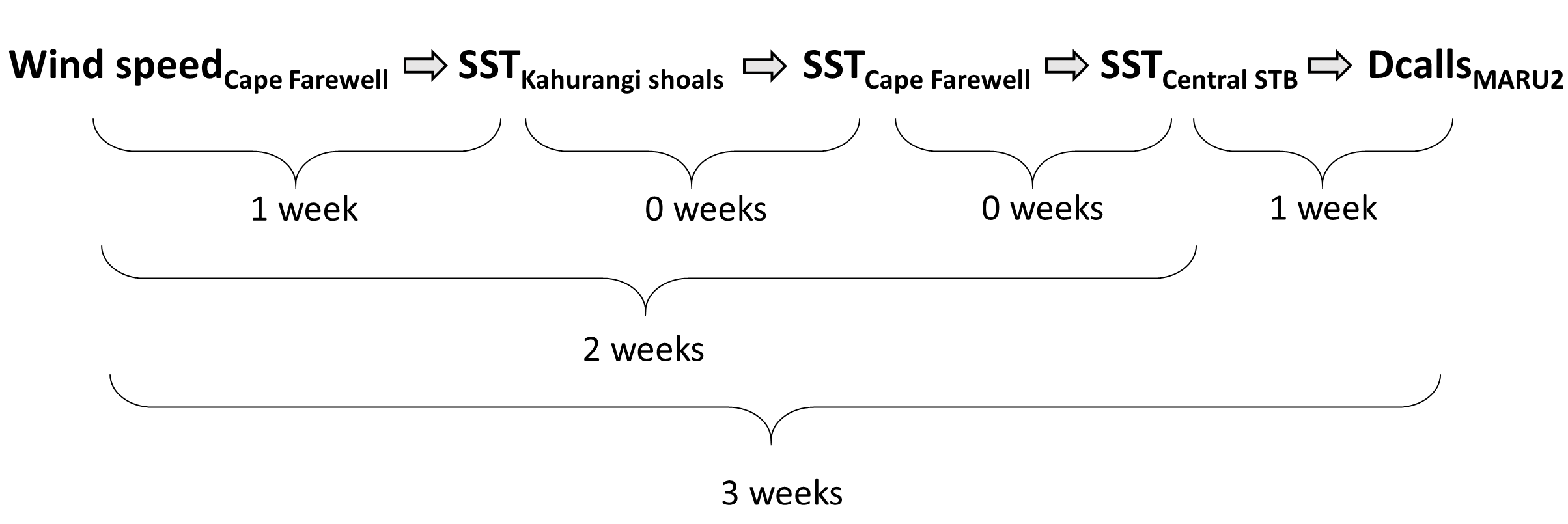
So, what did we find? It all starts with the wind. Wind instigates upwelling over an area off the northwest coast of the South Island of New Zealand called Kahurangi Shoals. This wind forcing spurs upwelling, leading to the formation of a cold water plume that propagates into the STB region, between the North and South Islands, with a lag of 1-2 weeks. Finally, we measured the density of blue whale vocalizations—sounds known as D calls, which are produced in a social context, and associated with foraging behavior—recorded at a hydrophone downstream along the upwelling plume’s path. D call density increased 3 weeks after increased wind speeds near the upwelling source. Furthermore, we looked at the lag time between wind events and aggregations in blue whale sightings. Blue whale aggregations followed wind events with a mean lag of 2.09 ± 0.43 weeks, which fits within our findings from the timeseries analysis. However, lag time between wind and whales is variable. Sometimes it takes many weeks following a wind event for an aggregation to form, other times mere days. The variability in lag can be explained by the amount of prior wind input in the system. If it has recently been windy, the water column is more likely to already be well-mixed and productive, and so whale aggregations will follow wind events with a shorter lag time than if there has been a long period without wind and the water column is stratified.
Figure 2. Top panel: Map of the study region within the South Taranaki Bight (STB) of New Zealand, with location denoted by the white rectangle on inset map in the upper right panel. All spatial sampling locations for sea surface temperature implemented in our timeseries analyses are denoted by the boxes, with the four focal boxes shown in white that represent the typical path of the upwelling plume originating off Kahurangi shoals and moving north and east into the STB. The purple triangle represents the Farewell Spit weather station where wind measurements were acquired. The location of the focal hydrophone (MARU2) where blue whale D calls were recorded is shown by the green star. (Reproduced from Barlow et al. 2021). Bottom panel: Results of the timeseries cross-correlation analyses, illustrating the lag between some of the metrics and locations examined.
This publication forms the second chapter of my PhD dissertation. However, in reality it is the culmination of a team effort. Just as whale aggregations lag wind events, publications lag years of hard work. The GEMM Lab has been studying New Zealand blue whales since Leigh first hypothesized that the STB was an undocumented foraging ground in 2013. I was fortunate enough to join the research effort in 2016, first as a Masters student and now as a PhD Candidate. I remember standing on the flying bridge of R/V Star Keys in New Zealand in 2017, when early in our field season we saw very few blue whales. Leigh and I were discussing this, with some frustration. Exclamations of “This is cold, upwelled water! Where are the whales?!” were followed by musings of “There must be a lag… It has to take some time for the whales to respond.” In summer 2019, Christina Garvey came to the GEMM Lab as an intern through the NSF Research Experience for Undergraduates program. She did an outstanding job of wrangling remote sensing and blue whale sighting data, and together we took on learning and understanding timeseries analysis to quantify lag. In a meeting with my PhD committee last spring where I presented preliminary results, Holger Klinck chimed in with “These results are interesting, but why haven’t you incorporated the acoustic data? That is a whale timeseries right there and would really add to your analysis”. Dimitri Ponirakis expertly computed the detection area of our hydrophone so we could adequately estimate the density of blue whale calls. Piecing everything together, and with advice and feedback from my PhD committee and many others, we now have a compelling and quantitative understanding of the upwelling dynamics in the STB ecosystem, and have thoroughly described the pathway from wind to whales in the region.
Figure 3. Dawn and Leigh on the flying bridge of R/V Star Keys on a windy day in New Zealand during the 2017 field season. Photo: T. Chandler.
Our findings are exciting, and perhaps even more exciting are the implications. Understanding the typical patterns that follow a wind event and how the upwelling plume propagates enables us to anticipate what will happen one, two, or up to three weeks in the future based on current conditions. These spatial and temporal lags between wind, upwelling, productivity, and blue whale foraging opportunities can be harnessed to generate informed forecasts of blue whale distribution in the region. I am thrilled to see this work in print, and equally thrilled to build on these findings to predict blue whale occurrence patterns.
Reference: Barlow, D.R., Klinck, H., Ponirakis, D., Garvey, C., Torres, L.G. Temporal and spatial lags between wind, coastal upwelling, and blue whale occurrence. Sci Rep 11, 6915 (2021). https://doi.org/10.1038/s41598-021-86403-y
In September of 2016, Leigh Torres, associate professor at Oregon State University, and I attended the 6th International Albatross and Petrel Conference. Somehow, amid all of the science that filled the week, Leigh first saw the Global Fishing Watch fishing map. She shouted with joy. She immediately envisioned a study to assess interactions between seabirds and fishing boats, and started considering a spatial overlap analysis between telemetry tracks of albatross with the Global Fishing Watch database. Such a study could help reduce bycatch, or the incidental catch of non-target species, like seabirds, in fisheries. Five years later, we executed that study in partnership with Global Fishing Watch, one of the first to look at fine-scale overlap between fishing vessels and marine life on the high seas (Orben et al. 2021).
Transparent data means opportunity for analysis
Despite knowing that bycatch from fisheries is a real, significant problem for many albatross populations, we have long struggled to know where birds go, where boats fish, and where the two interact in the vast ocean, especially in largely unregulated international waters. Albatross are long-lived seabirds and 15 out of the 22 species are threatened with extinction. Scientists have been tracking albatross for three decades, but assessing individual seabird encounters with vessels has traditionally been limited by a lack of transparency in fishing activity data. Some seabirds are attracted to fishing vessels because of the bait and offal, but we don’t know the whole story of why some birds approach vessels while others don’t.
When we first put our relatively large datasets together – 9,992 days of albatross tracking data from 150 birds and Global Fishing Watch fishing effort data from 2012-2016 – we weren’t sure what we would find. The ocean is a big place, and so finding where one bird and one vessel overlap is kind of like trying to find a needle in a haystack. Would we have enough encounters between birds and boats for an analysis? Would birds encounter fishing vessels as often as we think?
Measuring encounters between albatross and vessels
After overlaying the tracking data with a gridded daily layer of fishing effort, we identified potential encounters between birds and fishing boats. We identified when an albatross could detect a vessel, at a radius or 30 kilometers, and when an albatross had a close encounter with a vessel, within a radius of 3 kilometers (following methods developed in Collet Patrick & Weimerskirch, 2015). Then, we investigated factors that influenced the occurrence and duration of close encounters, considering the bird’s behavior, environmental conditions and habitat, fishing vessel and fisheries characteristics, and temporal variables, such as time of day and month.
Species variation of encounters
We conducted our analysis for three species of albatross that forage in the north Pacific ocean, Laysan albatross, black-footed albatross, and short-tailed albatross.
Adult black-footed albatrosses approached vessels for a close encounter 61.9 percent of the time they detected a fishing vessel.
Adult Laysan albatross had close encounters with a fishing boat 35.7 percent of the time they detected a vessel.
Juvenile short-tailed albatross had a lower frequency of close encounters (28.6 percent),
Understanding close encounters and their duration
Due to a low sample size of encounters, we were unable to investigate the reason for close encounters or their duration for black-footed albatrosses. More tracking data is critical to understand factors influencing the impact of vessels on this vulnerable species.
Laysan albatross were more likely to approach fishing vessels when fishing effort was high, but fishing boat density was low. Laysan albatross also had close encounters with vessels more frequently while they were foraging. Due to sample size, we could not further investigate the reason for the duration of encounters for this species.
Short-tailed albatrosses were also more likely to approach fishing vessels when they were searching for prey, fishing effort was high, and fishing boat density was low. They were more likely to have close encounters with vessels during the day and in habitats with water depths from 75-1500 meters.
Vessel attendance by short-tailed albatrosses was longer when sea surface temperatures were warmer and less productive, and during periods with lower wind speeds.
A useful approach
The information available to fisheries managers in order to reduce bycatch is most often limited to data collected from the perspective of the fishing vessels. Our analysis provides an alternative view – an albatross’ view of when and where boats are encountered in the seascape. While our analysis didn’t specifically look at bycatch, our estimates of proximity between birds and boats can be considered a proxy for increased bycatch risk.
For the endangered short-tailed albatross, bycatch events are few, but they come with high consequences for the bird population and fishing industry. Extending our study in a dynamic ocean management framework to provide an early warning system to predict when short-tailed albatross might make close and longer encounters with fishing vessels could be the next step. Furthermore, our analysis methods to assess when, where and why marine animals interact with fishing vessels can be applied to many other marine species in order to understand and reduce conflicts with fisheries.
This blog was for the Global Fishing Watch blog at globalfishingwatch.org
References
Collet, J., Patrick, S. C., & Weimerskirch, H. (2015). Albatrosses redirect flight towards vessels at the limit of their visual range. Marine Ecology Progress Series, 526, 199–205. http://doi.org/10.3354/meps11233
Orben, RA J Adams, M Hester, SA Shaffer, R Suryan, T Deguchi, K Ozaki, F Sato, LC Young, C Clatterbuck, MG Conners, DA Kroodsma, LG Torres. 2021. Across borders: External factors and prior behavior influence North Pacific albatross associations with fishing vessels. Journal of Applied Ecology. https://besjournals.onlinelibrary.wiley.com/doi/10.1111/1365-2664.13849
Last week marked the one year anniversary of the pandemic reality we have all been living. It has been an extremely challenging year, with everyone experiencing different kinds of difficulties and hurdles. One challenge that likely unites the majority of us is having to forego seeing our loved ones. For me personally, this is the longest time I have not seen my family (445 days and counting) and I know I am not alone in this situation. My homesickness started a train of thought about cetacean parental care and inspired me to write a blog about this topic. As you can see from the title, this post focuses on maternal care, rather than parental care. This bias isn’t due to my lack of research on this topic or active exclusion, but rather because there are currently no known cetacean species where paternal participation in offspring production and development extends beyond copulation (Rendell et al. 2019). Thus, this blog is all about the role of mothers in the lives of cetacean calves.
Like humans, cetacean mothers invest a lot of energy into their offspring. Most species have a gestation period of 10 or more months (Oftedal 1997). For baleen whale females in particular, pregnancy is not an easy feat given that they only feed during summer feeding seasons. They must therefore acquire all of the energy they will need for two migrations, birth, and (almost) complete lactation, before they will have access to food on feeding grounds again. For pregnant gray whales, a mere 4% loss in average energy intake on the foraging grounds will prevent her from successfully producing and/or weaning a calf (Villegas-Amtmann et al. 2015), demonstrating how crucial the foraging season is for a pregnant baleen whale. Once a calf is born, lactation ensues, ranging in length between approximately 6-8 months for most baleen whale species to upwards of one or two years in odontocetes (Oftedal 1997). The very short lactation period in baleen whales is offset by the large volume (for blue whales, up to 220 kg per day) and high fat percentage (30-50%) of milk that mothers provide for their calves (Oftedal 1997). In contrast, odontocetes (or toothed whales) have a more prolonged period of lactation with less fatty milk (10-30%). This discrepancy in lactation period lengths is in part because odontocete species do not undertake long migrations, which allows females to feed year-round and therefore allocate energy to nursing young for a longer time.
Blue whale calf nursing in New Zealand in 2016. Footage captured via unmanned aerial system (UAS; drone) piloted by Todd Chandler for GEMM Lab’s OBSIDIAN project. Source: GEMM Lab.
Aside from the energetically costly task of lactation, cetacean mothers must also assist their calves as they learn to swim. Echelon swimming is a common position of mother-calf pairs whereby the calf is in very close proximity to its mother’s mid-lateral flank and provides calves with hydrodynamic benefits. Studies in bottlenose dolphins have shown that swimming in echelon results in a 24% reduction in mean maximum swim speeds and a 13% decrease in distance per stroke (Noren 2008) for mothers, while concurrently increasing average swim speeds and distance per stroke of calves by 28% and 19%, respectively (Noren et al. 2007). While these studies have only been conducted in odontocete species, echelon swimming is also observed in baleen whales (Smultea et al. 2017), indicating that baleen whale females may experience the same reductions in swimming efficiency. Furthermore, mothers will forgo sleep in the first days after birth (killer whales & bottlenose dolphins; Lyamin et al. 2005) and/or shorten their dive foraging times to accommodate calf diving ability (bottlenose dolphins [Miketa et al. 2018] & belugas [Heide-Jørgensen et al. 2001]). Females must endure these losses in foraging opportunities and decreased swimming efficiency when they are at their most nutritionally stressed to ensure the well-being and success of their offspring.
It is at the time of weaning (when a calf becomes independent), that we start to see differences in the maternal role between baleen and toothed whale mothers. Odontocetes have much stronger sociality than baleen whales causing offspring to stay with their mothers for much longer periods. Among the largest toothed whales, such as killer and sperm whales, offspring stay with their mothers in stable matrilineal units for often a lifetime. Among the smaller toothed whales, such as bottlenose dolphins, maternal kin maintain strong bonds in dynamic fission-fusion societies. In contrast, post-weaning maternal care in baleen whales is limited, with the mother-calf pair typically separating soon after the calf is weaned (Rendell et al. 2019).
Conceptual diagram depicting where baleen (Mysticeti) and toothed (Odontoceti) whales fall on the continuum of low to high social structure and matrilineal kinship structure. The networks at the top depict long-term datasets of photo-identified individuals (red nodes = females, blue nodes = males, yellow nodes = calves) with thickness of connecting lines representing strength of association between individuals. Figure and caption [adapted] from Rendell et al. 2019.
The long-term impact of social bonds in odontocetes is evident through examples of vertically transmitted behaviors (from mother to calf) in a number of species. For example, the use of three unique foraging tactics (sponge carrying, rooster-tail foraging, and mill foraging) by bottlenose dolphin calves in Shark Bay, Australia, was only significantly explained by maternal use of these tactics (Sargeant & Mann 2009). In Brazil, individuals of four bottlenose dolphin populations along the coast cooperatively forage with artisanal fishermen, which involves specialized and coordinated behaviors from both species. This cooperative foraging tactic among dolphins is primarily maintained across generations via social learning from mothers to calves (Simões-Lopeset al. 2016). The risky tactic of intentional stranding by killer whales on beaches to capture elephant seal pups requires a high degree of skill and high parental investment to reduce the associated risk of stranding (Guinet & Bouvier 1995).
Evidence for vertical transmission of specialized foraging tactics in baleen whales currently does not exist. Bubble-net feeding is a specialized tactic employed by humpback whales in three oceanic regions where multiple individuals work together to herd and trap prey (Wiley et al. 2011). However, it remains unknown whether this behavior is vertically transmitted. Simultaneous video tags from a mother-calf humpback whale pair in the Western Antarctic Peninsula documented synchrony in dives, with the calf’s track lagging behind the mother’s by 4.5 seconds, suggesting that the calf was following its mother (Tyson et al. 2012). Synchronous diving likely allows calves to observe their mothers and practice their diving, and could offer a pathway for them to mimic foraging behaviors and tactics displayed by mothers.
While there currently may not be evidence for vertical transmission of specialized foraging tactics among the baleen whales, there is documentation of matrilineal fidelity to both foraging (Weinrich 1998, Barendse et al. 2013, Burnham & Duffus 2020) and breeding grounds (Carroll et al. 2015). Matrilineal site fidelity to foraging grounds is not exclusive to baleen whales and has also been documented in a number of odontocete species (Palsbøll et al. 1997, Turgeon et al. 2012).
A gallery of some GEMM Lab documented mother-calf gray whale pairs. All images captured under NOAA/NMFS permit #21678. Exclamation (mom; left) and Angie (calf; right).
Scarlett (mom; left) and Brown (calf; right).
Clouds (mom; back) and Cheetah (calf; front).
Xena (mom; back) and Evie (calf; front).
Knife (mom; left) and Daffodil (calf; right).
Pristine (mom; front) and Three Stars (calf; back).
Triplet (mom; right) and White Knuckle (calf; left).
In the GEMM Lab, we are interested in exploring the potential long-term bonds, role and impact of Pacific Coast Feeding Group (PCFG) gray whale mothers on their calves. GEMM Lab PhD student Clara Bird is digging into whether specialized foraging tactics, such as bubble blasts and headstands, are passed down from mothers to calves. I hope to assess whether using the PCFG range as a foraging ground (rather than the Arctic region) is a vertically transmitted behavior or whether environmental factors may play a larger role in the recruitment and dynamics of the PCFG. It will take us a while to get to the bottom of these questions, so in the meantime hug your loved ones if it’s safe to do so or, if you’re in my boat, continue to talk to them virtually until it is safe to be reunited.
References
Barendse, J., Best, P. B., Carvalho, I., and C. Pomilla. 2013. Mother knows best: occurrence and associations of resighted humpback whales suggest maternally derived fidelity to a southern hemisphere coastal feeding ground. PloS ONE 8:e81238.
Burnham, R. E., and D. A. Duffus. 2020. Maternal behaviors of gray whales (Eschrichtius robustus) on a summer foraging site. Marine Mammal Science 36:1212-1230.
Carroll, E. L., Baker, C. S., Watson, M., Alderman, R., Bannister, J., Gaggiotti, O. E., Gröcke, D. R., Patenaude, N., and R. Harcourt. 2015. Cultural traditions across a migratory network shape the genetic structure of southern right whales around Australia and New Zealand. Scientific Reports 5:16182.
Guinet, C., and J. Bouvier. 1995. Development of intentional stranding hunting techniques in killer whale (Orcinus orca) calves at Crozet Archipelago. Canadian Journal of Zoology 73:27-33.
Heide-Jørgensen, M. P., Hammeken, N., Dietz, R., Orr, J., and P. R. Richard. 2001. Surfacing times and dive rates for narwhals and belugas. Arctic 54:207-355.
Lyamin, O., Pryaslova, J., Lance, V., and J. Siegel. 2005. Continuous activity in cetaceans after birth. Nature 435:1177.
Miketa, M. L., Patterson, E. M., Krzyszczyk, E., Foroughirad, V., and J. Mann. 2018. Calf age and sex affect maternal diving behavior in Shark Bay bottlenose dolphins. Animal Behavior 137:107-117.
Noren, S. R. 2008. Infant carrying behavior in dolphins: costly parental care in an aquatic environment. Functional Ecology 22:284-288.
Noren, S. R., Biedenbach, F., Redfern, J. V., and E. F. Edwards. 2007. Hitching a ride: the formation locomotion strategy of dolphin calves. Functional Ecology 22:278-283.
Oftedal, O. T. Lactation in whales and dolphins: evidence of divergence between baleen- and toothed-species. Journal of Mammary Gland Biology and Neoplasia 2:205-230.
Palsbøll, P. J., Heide-Jørgensen, M. P., and R. Dietz. 1996. Population structure and seasonal movements of narwhals, Monodon monoceros, determined from mtDNA analysis. Heredity 78:284-292.
Rendell, L., Cantor, M., Gero, S., Whitehead, H., and J. Mann. 2019. Causes and consequences of female centrality in cetacean societies. Philosophical Transactions of the Royal Society B 374:20180066.
Sargeant, B. L., and J. Mann. 2009. Developmental evidence for foraging traditions in wild bottlenose dolphins. Animal Behavior 78:715-721.
Simões-Lopes, P. C., Daura-Jorge, F. G., and M. Cantor. 2016. Clues of cultural transmission in cooperative foraging between artisanal fishermen and bottlenose dolphins, Tursiops truncatus (Cetacea: Delphinidae). Zoologia (Curitiba) 33:e20160107.
Smultea, M. A., Fertl, D., Bacon, C. E., Moore, M. R., James, V. R., and B. Würsig. 2017. Cetacean mother-calf behavior observed from a small aircraft off Southern California. Animal Behavior and Cognition 4:1-23.
Turgeon, J., Duchesne, P., Colbeck, G. J., Postma, L. D., and M. O. Hammill. 2011. Spatiotemporal segregation among summer stocks of beluga (Delphinapterus leucas) despite nuclear gene flow: implication for the endangered belugas in eastern Hudson Bay (Canada). Conservation Genetics 13:419-433.
Tyson, R. B., Friedlaender, A. S., Ware, C., Stimpert, A. K., and D. P. Nowacek. 2012. Synchronous mother and calf foraging behaviour in humpback whales Megaptera novaeangliae: insights from multi-sensor suction cup tags. Marine Ecology Progress Series 457:209-220.
Villegas-Amtmann, S., Schwarz, L. K., Sumich, J. L., and D. P. Costa. 2015. A bioenergetics model to evaluate demographic consequences of disturbance in marine mammals applied to gray whales. Ecosphere 6:1-19.
Weinrich, M. 1998. Early experience in habitat choice by humpback whales (Megaptera novaeaengliae). Journal of Mammalogy 79:163-170.
Wiley, D., Ware, C., Bocconcelli, A., Cholewiak, D., Friedlaender, A., Thompson, M., and M. Weinrich. 2011. Underwater components of humpback whale bubble-net feeding behavior. Behavior 148:575-602.
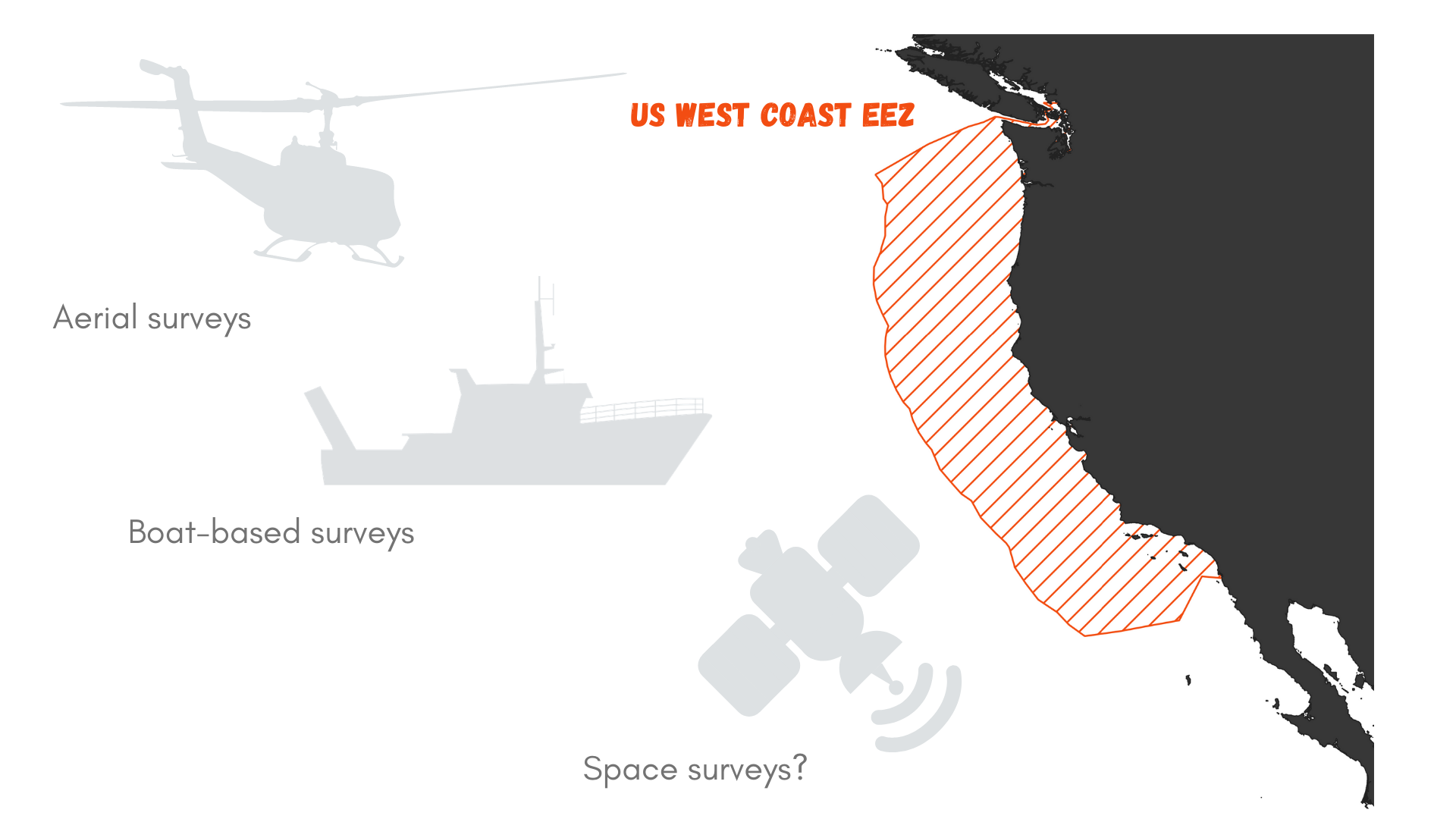
What I mean is that the vastness of the ocean is very hard to mentally visualize. When facing a conservation issue such as increased whale entanglement along the US West Coast (see OPAL project ), a tempting solution may be to suggest « let’s go see where the whales are and report their location to the fishermen?! ». But, it only takes a little calculation to realize how impractical this idea is.
Let’s roll out the numbers. The US West Coast exclusive economic zone (EEZ) stretches from the coast out to 200 nautical miles offshore, as prescribed by the 1982 United Nations Convention on the Law of the Sea. It covers an area of 825,549 km² (Figure 1). Now, imagine that you wish to survey this area for marine mammals. Using a vessel such as the R/V Bell M. Shimada that is used for the Northern California Current Ecosystem surveys cruises (NCC cruises, see Dawn and Rachel’s last blog), we may detect whales at a distance of roughly 6 km (based on my preliminary results). This distance of detection depends on the height of the observer, hence the height of the flying bridge where she/he is standing (the observer’s height may also be accounted for, but unless she/he is a professional basket-ball player, I think it can be neglected here). The Shimada is quite a large ship and it’s flying bridge is 13 meters above the water. Two observers may survey the water on each side of the trackline.
Considering that the vessel is moving at 8 knots (~15 km/h), we may expect to be effectively surveying 180 km² per hour (6x2x15). That’s not too bad, right?
Again, perspective is the key. If we divide the West Coast EEZ surface by 180 km² we can estimate that it would take 2,752 hours to survey this entire region. With an average of 12 hours of daylight, this takes us to…
382 DAYS OF SURVEY, searching for marine mammals over the US West Coast. Considering that observations cannot be undertaken on days with bad weather (fog, heavy rain, strong winds…), it might take more than a year and a half to complete the survey! And what would the marine mammals have done in the meantime? Move…
This little math exercise proves that exhaustively searching for the needle in the haystack from a vessel is not the way to go if we are to describe whale distribution and help mitigate the risk of entanglement. And using another platform of observation is not necessarily the solution. The OPAL project has relied on a great collaboration with the United States Coast Guard to survey Oregon waters. The USCG helicopters travel fast compared to a vessel, about 90 knots (167 km/h). As a result, more ground is covered but the speed at which it is traveling prevents the observer from detecting whales that are very far away. Based on the last analysis I ran for the OPAL project, whales are usually detected up to 3 km from the helicopter (only 5 % of sightings exceed that distance). In addition, the helicopter generally only has capacity for one observer at a time.
If we replicate the survey time calculation from above for the USCG helicopter, we realize that even with a fast-moving aerial survey platform it would still take 137 days to cover the West Coast EEZ.
Figure 1. What is the best survey method to document marine mammal occurrence in the US West Coast Exclusive Economic zone (EEZ)?
First, we can model and extrapolate. This approach is the path we are taking with the OPAL project: we survey Oregon waters in 4 different areas along the coast each month, then model observed whale densities as a function of topographic and oceanographic variables, and then predict whale probability of presence over the entire region. These predictions are based on the assumption that our survey design effectively sampled the variety of environmental conditions experienced by whales over the study region, which it certainly did considering that all sites are surveyed year-round.
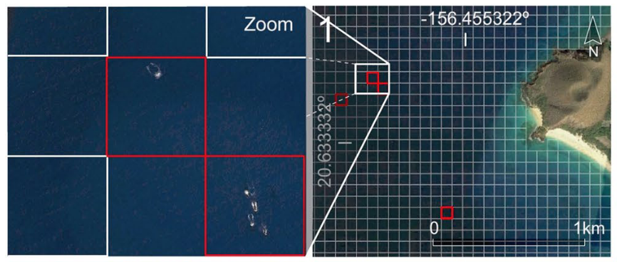
An alternative approach that has been recently discussed in the GEMM Llab, is the use of satellite images to detect whales along the coast. A communication entitled « The Potential of Satellite Imagery for Surveying Whales » was published last month in the Sensors Journal (Höschle et al., 2021) and presents the opportunities offered by this relatively new technology. The WorldView-3 satellite, owned by the company Digitalglobe and launched in 2016, has made it possible to commercialize imagery with a resolution never reached before, of the order of 30 cm per pixel. These very high resolution (VHR) satellite images make it possible to identify several species of large whales (Cubaynes et al. al., 2019) and to estimate their density (Bamford et al., 2020). Furthermore, machine learning algorithms, such as Neural Networks, have proved quite efficient at automatically detecting whales in satellite images (Guirado et al., 2019, Figure 2). While several new ultra-high resolution imaging satellites are expected to be launched in 2021 (by Maxar Technologies and Airbus), this “remote” approach looks like a promising avenue to detect whales over vast regions while drinking a cup of coffee at the office.
Figure 2. Illustration of a whale detection algorithm working on a gridded satellite image (DigitalGlobe). Source: Guirado et al., 2019.
But like any other data collection method, satellites have their drawbacks. We recently discovered that these VHR satellites are routinely switched off while passing above the ocean. Specific inquiries would need to be made to acquire data over our study areas, which would be at great expense. One of the cheapest provider I found is the Soar platform, that provides images at 50 cm resolution in partnership with the Chinese Aerospace Science and Technology Corporation. They advertise daily images anywhere on earth at $10 USD per km². This might sound cheap at first glance, but circling back to our US West Coast EEZ area calculations, we estimate that surveying this region entirely with satellite imagery would cost more than $8 million USD.
Yet, we have to look forward. The use of satellite imagery is likely to broaden and increase in the coming years, with a possible decrease in cost. Quoting Höschle et al. (2021) ‘To protect our world’s oceans, we need a global effort and we need to create opportunities for that to happen’.
Will satellites soon save whales?
References
Bamford, C. C. G. et al. A comparison of baleen whale density estimates derived from overlapping satellite imagery and a shipborne survey. Sci. Rep. 10, 1–12 (2020).
Cubaynes, H. C., Fretwell, P. T., Bamford, C., Gerrish, L. & Jackson, J. A. Whales from space: Four mysticete species described using new VHR satellite imagery. Mar. Mammal Sci. 35, 466–491 (2019).
Guirado, E., Tabik, S., Rivas, M. L., Alcaraz-Segura, D. & Herrera, F. Whale counting in satellite and aerial images with deep learning. Sci. Rep. 9, 1–12 (2019).
Höschle, C., Cubaynes, H. C., Clarke, P. J., Humphries, G. & Borowicz, A. The potential of satellite imagery for surveying whales. Sensors 21, 1–6 (2021).
Clara Bird, PhD Student, OSU Department of Fisheries and Wildlife, Geospatial Ecology of Marine Megafauna Lab
When I started working on my thesis, I anticipated many challenges related to studying the behavioral ecology of gray whales. From processing five-plus years of drone footage to data analysis, there has been no shortage of anticipated and unexpected issues. I recently hit an unexpected challenge when I started video processing that piqued my interest. As I’ve discussed in a previous blog, ethograms are lists of defined behaviors that help us properly and consistently collect data in a standardized approach. Ethograms form a crucial foundation of any behavior study as the behaviors defined ultimately affect what questions can be asked and what patterns are detected. Since I am working off of the thorough ethogram of Oregon gray whales from Torres et al. (2018), I had not given much thought to the process of adding behaviors to the ethogram. But, while processing the first chunk of drone videos, I noticed some behaviors that were not in the original ethogram and struggled to decide whether or not to add them. I learned that ethogram development can lead down several rabbit holes. The instinct to try and identify every movement is strong but dangerous. Every minute movement does not necessarily need to be included and it’s important to remember the ultimate goal of the analysis to avoid getting bogged down.
Fundamental behavior questions cannot be answered without ethograms. For example, Baker et al. (2017) developed an ethogram for bottlenose dolphins in Ireland in order to conduct an initial quantitative behavior analysis. They did so by reviewing published ethograms for bottlenose dolphins, consulting with multiple experts, and revising the ethogram throughout the study. They then used their data to test inter-observer variability, calculate activity budgets, and analyze how the activity budgets varied across space and time.
Howe et al. (2015) also developed an ethogram in order to conduct quantitative behavior analyses. Their goals were to use the ethogram and subsequent analyses to better understand the behavior of beluga whales in Cook Inlet, AK, USA and to inform conservation. They started by writing down all behaviors they observed in the field, then they consolidated their notes into a formal ethogram that they used and refined during subsequent field seasons. They used their data to analyze how the frequencies of different behaviors varied throughout the study area at different times. This study served as an initial analysis investigating the effect of anthropogenic disturbance and was refined in future studies.
My research is similarly geared towards understanding behavior patterns to ultimately inform conservation. The primary questions of my thesis involve individual specialization, patterns of behavior across space, the relationship between behavior and body condition, and social behavior (check out this blog to learn more). While deciding what behaviors to add to my ethogram I’ve had to remind myself of these main questions and the bigger picture. The drone footage lets us see so much detail that it’s tempting to try to define every movement we can observe. One rabbit hole I’ve had to avoid a few times is locomotion. From the footage, it is possible to document fluke beats and pectoral fin strokes. While it could be interesting to investigate how different whales move in different ways, it could easily become a complicated mess of classifying different movements and take me deep into the world of whale locomotion. Talking through what that work would look like reminded me that we cannot answer every question and trying to assess all exciting side projects can cause us to lose focus on the main questions.
While I avoided going down the locomotion rabbit hole, there were some new behaviors that I did add to my ethogram. I’ll illustrate the process with the examples of two new behaviors I recently added: fluke swish and pass under (Clips 1 and 2). Clip 1 shows a whale rapidly moving its fluke to the side. I chose to add fluke swish because it’s such a distinct movement and I’m curious to see if there’s a pattern across space, time, individual, or nearby human activity that might explain its function. Clip 2 shows a calf passing under its mom. It’s not nursing because the calf doesn’t spend time under its mom, it just crosses underneath her. The calf pass under behavior could be a type of mom-calf tactile interaction. Analyzing how the frequency of this behavior changes over time could show how a calf’s dependency on its mom changes over as it ages.
In defining these behaviors, I had to consider how many different variations of this behavior would be included in the definition. This process involves considering at what point a variation of that behavior could serve a different function, even without knowing the function of the original behavior. For fluke swish this process involved deciding to only count a behavior as a fluke swish if it was a big, fast movement. A small and slow movement of the fluke a little to the side could serve a different function, such as turning, or be a random movement.
Clip 1: Fluke swish behavior (Video filmed under NOAA/NMFS research permit #16111 by certified drone pilot Todd Chandler).
Clip 2: Pass under behavior (Video filmed under NOAA/NMFS research permit #16111 by certified drone pilot Todd Chandler).
The next step involved deciding if the behavior would be a ‘state’ or ‘point’ event. A state event is a behavior with a start and stop moment; a point event is instantaneous and assigned to just a point in time. I would categorize a behavior as a state event if I was interested in questions about its duration. For example, I could ask “what percentage of the total observation time was spent in a certain behavior state?” A point event would be a behavior where duration is not applicable, but I could ask a question like “Did whale 1 perform more point event A than whale 2?”. Both fluke swish and pass under are point events because they only happen for an instant. In a pass under the calf is passing under its mom for just a brief point in time, making it a point event. The final step was to name the behavior. As I discussed in this blog, the name of the behavior does not matter as much as the definition but it is important that the name is clear and descriptive. We chose the name fluke swish because the fluke rapidly moves from side to side and pass under because the calf crosses under its mom.
Frankly, in the beginning, I was a bit overwhelmed by the realization that the content of my ethogram would ultimately control the questions I could answer. I could not help but worry that after processing all the videos, I would end up regretting not defining more behaviors. However, after reading some of the literature, chatting with Leigh, and reviewing the initial chunk of videos several times, I am more confidence in my judgment and my ethogram. I have accepted the fact that I can’t anticipate everything, and I am confident that the behaviors I need to answer my research questions are included. The process of reviewing and updating my ethogram has been a rewarding challenge that resulted in a valuable lesson that I will take with me for the rest of my career.
References
Baker, I., O’Brien, J., McHugh, K., & Berrow, S. (2017). An ethogram for bottlenose dolphins (Tursiops truncatus) in the Shannon Estuary, Ireland. Aquatic Mammals, 43(6), 594–613. https://doi.org/10.1578/AM.43.6.2017.594
Howe, M., Castellote, M., Garner, C., McKee, P., Small, R. J., & Hobbs, R. (2015). Beluga, Delphinapterus leucas, ethogram: A tool for cook inlet beluga conservation? Marine Fisheries Review, 77(1), 32–40. https://doi.org/10.7755/MFR.77.1.3
Torres, L. G., Nieukirk, S. L., Lemos, L., & Chandler, T. E. (2018). Drone up! Quantifying whale behavior from a new perspective improves observational capacity. Frontiers in Marine Science, 5(SEP). https://doi.org/10.3389/fmars.2018.00319