By Natalie Nickells, visiting PhD Student, British Antarctic Survey
For the last three months, I’ve been lucky enough to be welcomed into the GEMM lab as a visiting PhD student to work on the acoustic data from hydrophones in CATS tags deployed on gray whales. This work has been a huge change for me! I’ve gone from studying Antarctic baleen whale foraging, the topic of my PhD, from a distance at my desk in Cambridge England, to studying PCFG gray whales in Newport- and finally being in the same country, state, and even county to the whales I am studying! Unlike my Antarctic research, where whale blows in the distance become tiny points in a sea of data, listening to the CATS tag data has allowed me to really connect with these animals on an emotional level, as I’ve spent days, weeks and months listening to the world as they hear it.
Humans are fundamentally visual creatures- we take in information through sight first, with hearing probably our second, or for some even third, sense in line. However, for marine mammals, the same cannot be said: their world is auditory first. This fact is an important realisation to get our heads around, highlighted beautifully by the phrase “the ears are the window to the soul of the whale” (Sonic Sea (2017)) or Tim Donaghy’s emotive statement that “a deaf whale is a dead whale”. High levels of ocean noise therefore have a huge impact on baleen whales. Imagine trying to do your groceries or find a friend while blindfolded or in a thick fog– you might struggle to access food or communicate with others, and your stress would certainly be high. To succeed, you would likely need to change your behaviour.
Behavioural changes in response to ocean noise are observed in baleen whales: for example, humpback whales change their foraging behaviour when ship noise increases (Blair et al., 2016), and gray whales have been shown to call more frequently and possibly more loudly in conditions of high ocean noise (Dahlheim & Castellote, 2016). However, even in the absence of notable behaviour change due to ocean noise, North Atlantic right whales may still be experiencing a stress response. When shipping traffic in the Bay of Fundy significantly decreased in the aftermath of 9/11, North Atlantic right whales in the area had decreased chronic stress levels (Rolland et al., 2012).
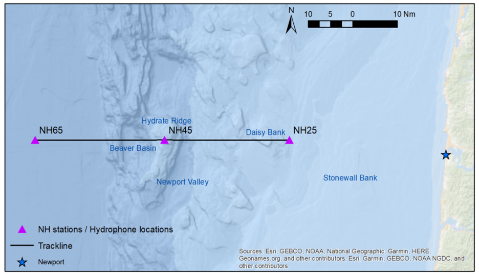
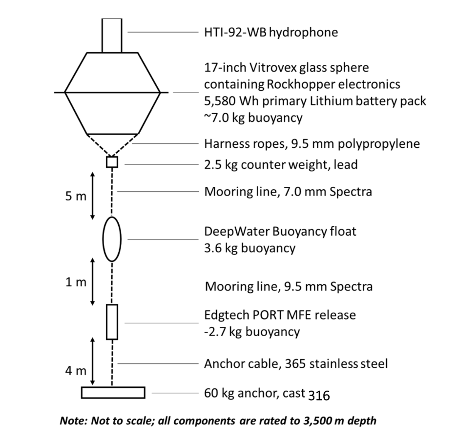
Previous work by the GEMM lab observed this stress response to ocean noise in gray whales. They found a correlation between high levels of glucocorticoid (a stress indicator) in male gray whale faeces with high vessel noise and vessel counts in the area. Vessel noise was measured using two static hydrophones off the Oregon coast, and it was assumed all animals in the area experienced the same noise (Lemos et al., 2022; Pirotta et al., 2023). However, a static hydrophone is an imperfect measure of the sound levels a mobile animal experiences, particularly as we might expect animals to change behaviour when disturbed (Sullivan & Torres, 2018). This previous work became the starting point for the question I have addressed during my time in the GEMM Lab: can we measure and characterise the sound levels an individual whale was exposed to? Enter CATS tags. These are suction-cup tags fitted with a host of sensors, which have been used by the GEMM lab since 2021 (see Image 1). So far, they have mostly been used for their accelerometry data (Colson et al. (in press), see also Kate’s blog post). However, the GEMM lab had the foresight to put hydrophones on these tags, and as a result I was welcomed into the lab by a bumper-crop of hydrophone data just waiting to be analysed!

This tag data is particularly valuable, not only for its ability to follow the acoustic world of an individual whale, but also due to the whole suite of data that comes with the acoustics: essentially, the acoustic data comes with behavioural data. Or at least, it comes with data from which we can infer behaviour (Colson et al, in press)! Incorporating behaviour into passive acoustics work hugely strengthens its ecological usefulness (Oestreich et al., 2024). We can hear what an individual whale is hearing, and we can also infer what they were doing before, during, and after they heard or made that sound. Having behavioural data also means that we can ground-truth the sounds we hear. When hearing an interesting sound, I can go back to the video data and accelerometer data to check what the whale sees, what its body-position is doing (e.g., is it headstand foraging?) and the speed and direction of its travel. Context is key!
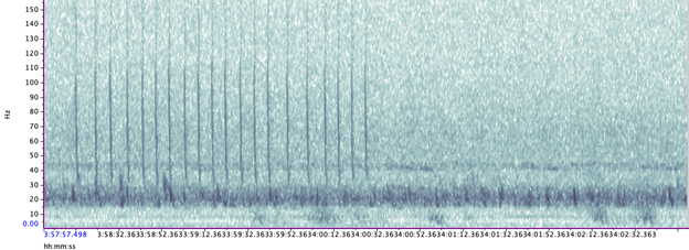
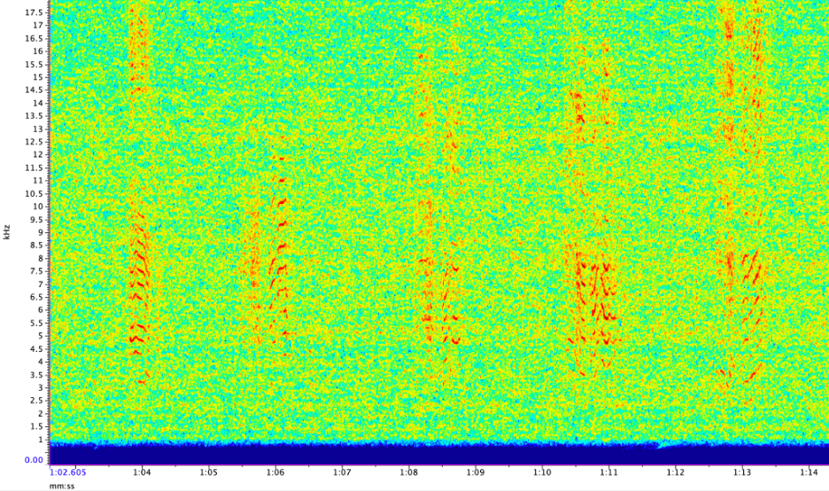
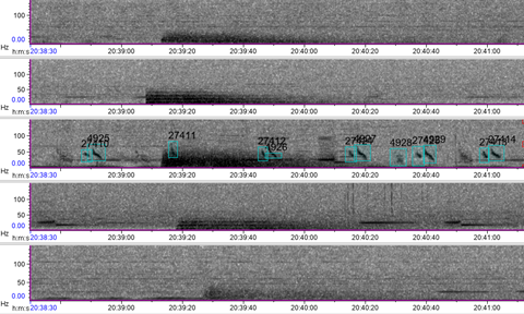
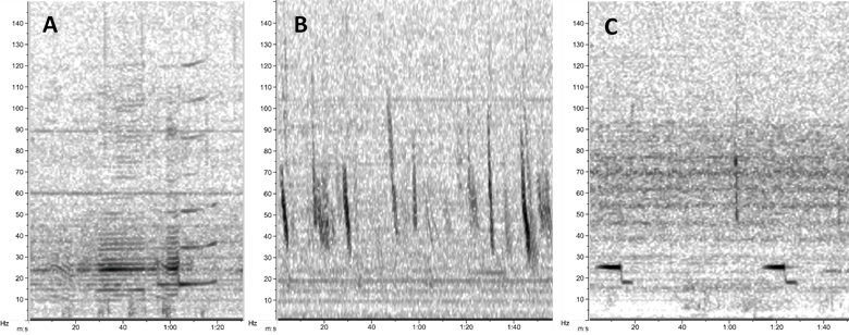
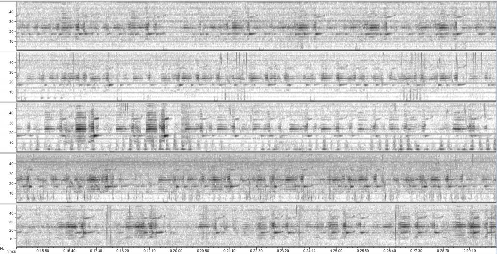
The importance of context was highlighted in my very first week here in the GEMM lab. I became very interested in a sound I could hear frequently when the whale would surface- a distorted bark-like noise, but the whale was surely too far offshore for any barking dog to be heard? And almost every time the whale surfaced? After a few days pondering, I shared my mystery with Leigh, who laughingly revealed that one of the whale-watching boats in this area has a ‘whale-alerting’ dog on board! Sometimes if it sounds like a dog… it’s a dog! Besides my slightly anticlimactic discovery of dogs barking, committing time to listening to the tags and hearing what the whales hear, has been a magical experience. My favourite hydrophone sound, that still gets me excited when I hear it, is the gray whale ‘bongo call’- or as it’s more formally known in the literature, M1 vocalisation (Guazzo et al., 2019). I’ll let you decide which name is more appropriate! I first heard this call when investigating a time on “Scarlett’s” tag when we knew her 14 year-old daughter “Pacman” had been close: about 15 minutes before “Pacman” appears on the video, Scarlett makes this call (you can play the clip below to listen). In “Lunita’s” tag, we even hear this call three times in a row!
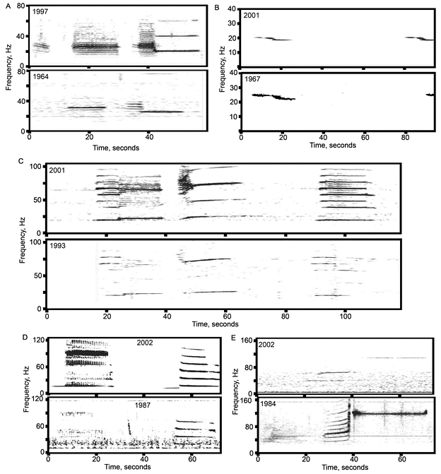
Relatively little research has been done on gray whale calls compared to other more studied species like humpbacks. Most of this research has taken place on gray whale migratory routes (Guazzo et al., 2019, 2017; Burnham et al. 2018) or in captivity (Fish et. al, 1974 ) so these tag recordings could be a valuable addition to a small sample from the foraging grounds (Clayton et al., 2023; Haver et al., 2023)- as well as being very personally exciting to hear!
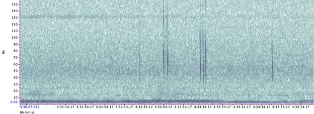
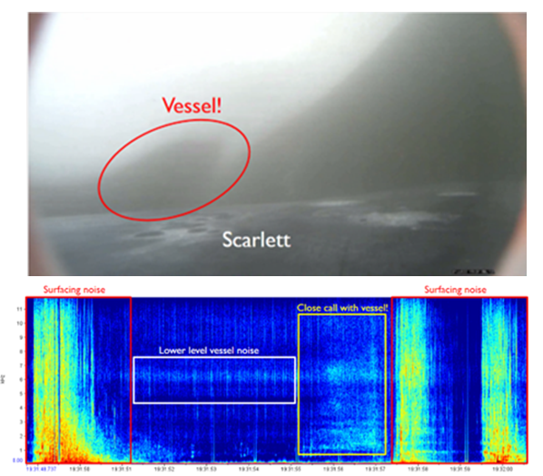
We’ve also been able to use the tag hydrophone data to look at close calls with ships. As I was going through the data on “Scarlett’s” tag, I noticed a spike in vessel noise. Looking at the video from the same timestamp, I could see a small vessel passing directly over her as she surfaced. At the time this vessel passed over her, the tag was only 0.8 m under the surface of the water!
Sometimes vessels may be more distant, but possibly equally harmful: we have seen vessel noise from larger and presumably more distant vessels dominate the soundscape in some of the tag data. Remembering that to a whale, the sonic world is as important as the visual world is to us, this elevated background noise from ships could have major consequences. So, the first step is to try to quantify the gray whales’ exposure to this vessel noise. I’ve been running some systematic sampling on the tag data to try to quantify background noise levels, and how this changes depending on the time of day: do individual whales experience the same daily spikes in ocean noise that were detected on the static hydrophones, at around 6am and noon due to vessel traffic (Haver et al., 2023)? If not, are they taking evasive action to avoid these spikes? These are just some of the questions that these CATS tags can help us answer, although ideally we need longer acoustic data recordings to capture day and night data, as well as potentially improving the hydrophones on the CATS tags themselves to minimise the impacts of tag interference and random noise.
When explaining to the public what it is to be a PhD student, I often refer to myself as a ‘scientist in training’, or to young children, a ‘baby scientist’. As I look toward my departure from the GEMM lab, I hope to have developed into at least a scientific toddler, having gained the ability to walk through reams of acoustic data with (relative) independence. More than that, I’m excited to take home a refreshed sense of curiosity about what drives marine mammals to behave as they do, an openness to collaboration and new approaches, and a large dose of ‘American emotion’! Let’s hope my British colleagues can handle it!
My heartfelt thanks to all those who welcomed me so warmly at the GEMM lab and Oregon State University, particularly my mentors Leigh Torres and Samara Haver.
Did you enjoy this blog? Want to learn more about marine life, research, and conservation? Subscribe to our blog and get a weekly alert when we make a new post! Just add your name into the subscribe box below!
Bibliography
Sonic Sea (2017) Directed by Michelle Dougherty [Film] Distributed by the Natural Resources Defense Council.
Blair, H.B., Merchant, N.D., Friedlaender, A.S., Wiley, D.N. & Parks, S.E. (2016) Evidence for ship noise impacts on humpback whale foraging behaviour. Biology Letters. 12 (8), 20160005. doi:10.1098/rsbl.2016.0005.
Burnham, R., Duffus, D. & Mouy, X. (2018) Gray Whale (Eschrictius robustus) Call Types Recorded During Migration off the West Coast of Vancouver Island. Frontiers in Marine Science. 5, 329. doi:10.3389/fmars.2018.00329.
Colson, K., E. Pirotta L. New, D Cade, J Calambokidis, K. Bierlich, C Bird, A Fernandez Ajó, L. Hildebrand, A. Trites, L. Torres. (in press). Using accelerometry tags to quantify gray whale foraging behavior. Marine Mammal Science.
Clayton, H., Cade, D.E., Burnham, R., Calambokidis, J. & Goldbogen, J. (2023) Acoustic behavior of gray whales tagged with biologging devices on foraging grounds. Frontiers in Marine Science. 10, 1111666. doi:10.3389/fmars.2023.1111666.
Dahlheim, M. & Castellote, M. (2016) Changes in the acoustic behavior of gray whales Eschrichtius robustus in response to noise. Endangered Species Research. 31, 227–242. doi:10.3354/esr00759.
Fish, J.F., Sumich, J.L. & Lingle, G.L. (n.d.) Sounds Produced by the Gray Whale, Eschrichtius robustus.
Guazzo, R., Schulman-Janiger, A., Smith, M., Barlow, J., D’Spain, G., Rimington, D. & Hildebrand, J. (2019) Gray whale migration patterns through the Southern California Bight from multi-year visual and acoustic monitoring. Marine Ecology Progress Series. 625, 181–203. doi:10.3354/meps12989.
Guazzo, R.A., Helble, T.A., D’Spain, G.L., Weller, D.W., Wiggins, S.M. & Hildebrand, J.A. (2017) Migratory behavior of eastern North Pacific gray whales tracked using a hydrophone array S. Li (ed.). PLOS ONE. 12 (10), e0185585. doi:10.1371/journal.pone.0185585.
Haver, S.M., Haxel, J., Dziak, R.P., Roche, L., Matsumoto, H., Hvidsten, C. & Torres, L.G. (2023) The variable influence of anthropogenic noise on summer season coastal underwater soundscapes near a port and marine reserve. Marine Pollution Bulletin. 194, 115406. doi:10.1016/j.marpolbul.2023.115406.
Lemos, L.S., Haxel, J.H., Olsen, A., Burnett, J.D., Smith, A., Chandler, T.E., Nieukirk, S.L., Larson, S.E., Hunt, K.E. & Torres, L.G. (2022) Effects of vessel traffic and ocean noise on gray whale stress hormones. Scientific Reports. 12 (1), 18580. doi:10.1038/s41598-022-14510-5.
Oestreich, W.K., Oliver, R.Y., Chapman, M.S., Go, M.C. & McKenna, M.F. (2024) Listening to animal behavior to understand changing ecosystems. Trends in Ecology & Evolution. S0169534724001459. doi:10.1016/j.tree.2024.06.007.
Pirotta, E., Fernandez Ajó, A., Bierlich, K.C., Bird, C.N., Buck, C.L., Haver, S.M., Haxel, J.H., Hildebrand, L., Hunt, K.E., Lemos, L.S., New, L. & Torres, L.G. (2023) Assessing variation in faecal glucocorticoid concentrations in gray whales exposed to anthropogenic stressors S. Cooke (ed.). Conservation Physiology. 11 (1), coad082. doi:10.1093/conphys/coad082.
Rolland, R.M., Parks, S.E., Hunt, K.E., Castellote, M., Corkeron, P.J., Nowacek, D.P., Wasser, S.K. & Kraus, S.D. (2012) Evidence that ship noise increases stress in right whales. Proceedings of the Royal Society B: Biological Sciences. 279 (1737), 2363–2368. doi:10.1098/rspb.2011.2429.
Sullivan, F.A. & Torres, L.G. (2018) Assessment of vessel disturbance to gray whales to inform sustainable ecotourism. The Journal of Wildlife Management. 82 (5), 896–905. doi:10.1002/jwmg.21462.