Can sea otters help kelp under a changing climate?

By Dominique Kone1 and Sara Hamilton2

1Masters Student in Marine Resource Management, 2Doctoral Student in Integrative Biology

Five years ago, the North Pacific Ocean experienced a sudden increase in sea surface temperature (SST), known as the warm blob, which altered marine ecosystem function and structure (Leising et al. 2015). Much research illustrated how the warm blob impacted pelagic ecosystems, with relatively less focused on the nearshore environment. Yet, a new study demonstrated how rising ocean temperatures have partially led to bull kelp loss in northern California. Unfortunately, we are once again observing similar warming trends, representing the second largest marine heatwave over recent decades, and signaling the potential rise of a second warm blob. Taken together, all these findings could forecast future warming-related ecosystem shifts in Oregon, highlighting the need for scientists and managers to consider strategies to prevent future kelp loss, such as reintroducing sea otters.

In northern California, researchers observed a dramatic ecosystem shift from productive bull kelp forests to purple sea urchin barrens. The study, led by Dr. Laura Rogers-Bennett from the University of California, Davis and California Department of Fish and Wildlife, determined that this shift was caused by multiple climatic and biological stressors. Beginning in 2013, sea star populations were decimated by sea star wasting disease (SSWD). Sea stars are a main predator of urchins, causing their absence to release purple urchins from predation pressure. Then, starting in 2014, ocean temperatures spiked with the warm blob. These two events created nutrient-poor conditions, which limited kelp growth and productivity, and allowed purple urchin populations to grow unchecked by predators and increase grazing on bull kelp. The combined effect led to approximately 90% reductions in bull kelp, with a reciprocal 60-fold increase in purple urchins (Figure 1).
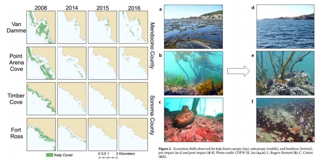
Figure 1. Kelp loss and ecosystem shifts in northern California (Rogers-Bennett & Catton 2019).

These changes have wrought economic challenges as well as ecological collapse in Northern California. Bull kelp is important habitat and food source for several species of economic importance including red abalone and red sea urchins (Tegner & Levin 1982). Without bull kelp, red abalone and red sea urchin populations have starved, resulting in the subsequent loss of the recreational red abalone ($44 million) and commercial red sea urchin fisheries in Northern California. With such large kelp reductions, purple urchins are also now in a starved state, evidenced by noticeably smaller gonads (Rogers-Bennett & Catton 2019).

Biogeographically, southern Oregon is very similar to northern California, as both are composed of complex rocky substrates and shorelines, bull kelp canopies, and benthic macroinvertebrates (i.e. sea urchins, abalone, etc.). Because Oregon was also impacted by the 2014-2015 warm blob and SSWD, we might expect to see a similar coastwide kelp forest loss along our southern coastline. The story is more complicated than that, however. For instance, ODFW has found purple urchin barrens where almost no kelp remains in some localized places. The GEMM Lab has video footage of purple urchins climbing up kelp stalks to graze within one of these barrens near Port Orford, OR (Figure 2, left). In her study, Dr. Rogers-Bennett explains that this aggressive sea urchin feeding strategy is potentially a sign of food limitation, where high-density urchin populations create intense resource competition. Conversely, at sites like Lighthouse Reef (~45 km from Port Orford) outside Charleston, OR, OSU and University of Oregon divers are currently seeing flourishing bull kelp forests. Urchins at this reef have fat, rich gonads, which is an indicator of high-quality nutrition (Figure 2, right).

Satellites can detect kelp on the surface of the water, giving scientists a way to track kelp extent over time. Preliminary results from Sara Hamilton’s Ph.D. thesis research finds that while some kelp forests have shrunk in past years, others are currently bigger than ever in the last 35 years. It is not clear what is driving this spatial variability in urchin and kelp populations, nor why southern Oregon has not yet faced the same kind of coastwide kelp forest collapse as northern California. Regardless, it is likely that kelp loss in both northern California and southern Oregon may be triggered and/or exacerbated by rising temperatures.
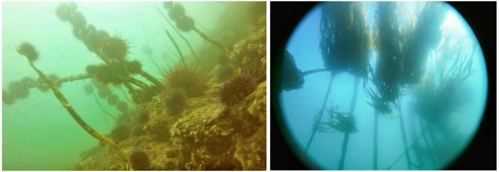
Figure 2. Left: Purple urchin aggressive grazing near Port Orford, OR (GEMM Lab 2019). Right: Flourishing bull kelp near Charleston, OR (Sara Hamilton 2019).

The reintroduction of sea otters has been proposed as a solution to combat rising urchin populations and bull kelp loss in Oregon. From an ecological perspective, there is some validity to this idea. Sea otters are a voracious urchin predator that routinely reduce urchin populations and alleviate herbivory on kelp (Estes & Palmisano 1974). Such restoration and protection of bull kelp could help prevent red abalone and red sea urchin starvation. Additionally, restoring apex predators and increasing species richness is often linked to increased ecosystem resilience, which is particularly important in the face of global anthropogenic change (Estes et al. 2011)

While sea otters could alleviate grazing pressure on Oregon’s bull kelp, this idea only looks at the issue from a top-down, not bottom-up, perspective. Sea otters require a lot of food (Costa 1978, Reidman & Estes 1990), and what they eat will always be a function of prey availability and quality (Ostfeld 1982). Just because urchins are available, doesn’t mean otters will eat them. In fact, sea otters prefer large and heavy (i.e. high gonad content) urchins (Ostfeld 1982). In the field, researchers have observed sea otters avoiding urchins at the center of urchin barrens (personal communication), presumably because those urchins have less access to kelp beds than on the barren periphery, and therefore, are constantly in a starved state (Konar & Estes 2003) (Figure 3). These findings suggest prey quality is more important to sea otter survival than just prey abundance.
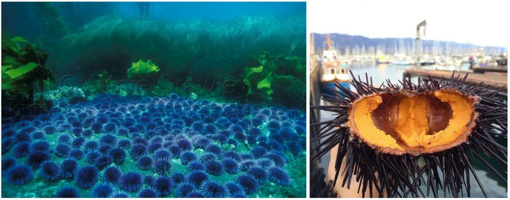
Figure 3. Left: Sea urchin barren (Annie Crawley). Right: Urchin gonads (Sea to Table).

Purple urchin quality has not been widely assessed in Oregon, but early results show that gonad size varies widely depending on urchin density and habitat type. In places where urchin barrens have formed, like Port Orford, purple urchins are likely starving and thus may be a poor source of nutrition for sea otters. Before we decide whether sea otters are a viable tool to combat kelp loss, prey surveys may need to be conducted to assess if a sea otter population could be sustained based on their caloric requirements. Furthermore, predictions of how these prey populations may change due to rising temperatures could help determine the potential for sea otters to become reestablished in Oregon under rapid environmental change.

Recent events in California could signal climate-driven processes that are already impacting some parts of Oregon and could become more widespread. Dr. Rogers-Bennett’s study is valuable as she has quantified and described ecosystem changes that might occur along Oregon’s southern coastline. The resurgence of a potential second warm blob and the frequency between these warming events begs the question if such temperature spikes are still anomalous or becoming the norm. If the latter, we could see more pronounced kelp loss and major shifts in nearshore ecosystem baselines, where function and structure is permanently altered. Whether reintroducing sea otters can prevent these changes will ultimately depend on prey and habitat availability and quality, and should be carefully considered.

References:

Costa, D. P. 1978. The ecological energetics, water, and electrolyte balance of the California sea otter (Enhydra lutris). Ph.D. dissertation, University of California, Santa Cruz.

Estes, J. A. and J.F. Palmisano. 1974. Sea otters: their role in structuring nearshore communities. Science. 185(4156): 1058-1060.

Estes et al. 2011. Trophic downgrading of planet Earth. Science. 333(6040): 301-306.

Harvell et al. 2019. Disease epidemic and a marine heat wave are associated with the continental-scale collapse of a pivotal predator (Pycnopodia helianthoides). Science Advances. 5(1).

Konar, B., and J. A. Estes. 2003. The stability of boundary regions between kelp beds and deforested areas. Ecology. 84(1): 174-185.

Leising et al. 2015. State of California Current 2014-2015: impacts of the warm-water “blob”. CalCOFI Reports. (56): 31-68.

Ostfeld, R. S. 1982. Foraging strategies and prey switching in the California sea otter. Oecologia. 53(2): 170-178.

Reidman, M. L. and J. A. Estes. 1990. The sea otter (Enhydra lutris): behavior, ecology, and natural history. United States Department of the Interior, Fish and Wildlife Service, Biological Report. 90: 1-126.

Rogers-Bennett, L., and C. A. Catton. 2019. Marine heat wave and multiple stressors tip bull kelp forest to sea urchin barrens. Scientific Reports. 9:15050.

Tegner, M. J., and L. A. Levin. 1982. Do sea urchins and abalones compete in California? International Echinoderms Conference, Tampa Bay. J. M Lawrence, ed.

Whispers of fear

By Leila S. Lemos, Ph.D. candidate in Wildlife Sciences, Fisheries and Wildlife Department


What did you do when playing hide-and-seek? You would try your best not to move or make any noise that would cause the seeker to hear you and find you, right? So, I always associated the prey-predator relationship to a hide-and-seek game, where prey hide, and predators seek. Thus, if you are the prey in this food chain game you should try to hide and not make any noise.

I read an article last week that made me think of this relationship again. The article, “Right whale moms ‘whisper’ to their babies so sharks won’t hear”, announced the study findings from Susan E. Parks and collaborators (2019), which really called my attention.

To give some context, North Atlantic Right Whales (NARWs; Eubalaena glacialis; Fig. 1) occur primarily in northern Atlantic coastal waters or close to the continental shelf (Fig. 2), yet their presence in deep waters are also known (NOAA 2019).

Figure 1: A mother-calf pair of North Atlantic right whales.
Source: Dana Cusano, Syracuse University (NMFS Permit #775-1875); retrieved from Kooser 2019.

Figure 2: North Atlantic right whale distribution.
Source: NOAA 2019.

The species is critically endangered and estimated at less than 500 individuals (IUCN 2007, Pace et al. 2017). Unlike several other whale populations, NARWs have not rebounded from intense whaling, and its population has begun to decrease since 2010 (Thomas et al. 2016, Pace et al. 2017). NARWs’ biggest threats are associated with anthropogenic activities, including entanglement in fishing lines and collisions with vessels (Fig. 3).

Figure 3: North Atlantic right whales’ biggest threats: (A) entanglement in fishing gear, and (B) vessel collision.
Source (A): Peter Duley (NOAA), retrieved from Guy 2017; (B) Williams 2019.

Other than anthropogenic impacts, NARWs also face natural threats like predation. There are reports on newborn and young right whale calf’s predation by killer whales and large sharks (Taylor et al. 2013, Parks et al. 2019; Fig. 4).

Figure 4: Mother carries her calf carcass presenting two semicircular shark bite marks on its flank.
Source: Taylor et al. 2013.

Whales communicate by acoustic signals that can efficiently propagate underwater and be detected by listening predators (Parks et al. 2019). It is possible that mother-calf pairs may use cryptic behaviors to avoid the attention of predators by shifting their communication patterns, leading to a hypothesis that they produce low-amplitude calls and lower call rates (Tyack 2000; Fig. 5). These two behavioral modifications have been previously observed in mother-calf pairs of humpback whales (Megaptera novaeangliae; Videsen et al. 2017) and southern right whales (Eubalaena australis; Nielsen et al. 2019).

Figure 5: Spectrogram and waveform of a single pulse (low amplitude) and an upcall (high amplitude) produced by a right whale. A louder and longer signal (high-amplitude call) is potentially easier to detect by predators.
Source: Parks et al. 2019.

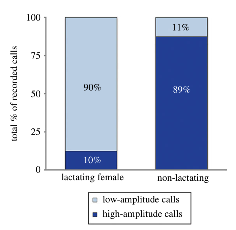
In order to determine if NARWs exhibited the same behavior, Parks and collaborators (2019) tagged lactating and non-lactating females, and a pregnant female that later was tagged again with her calf, to collect acoustic, movement and orientation data. Their results indicate that lactating females use a significantly higher low-amplitude call rate (mean ± standard deviation: 7.13 ± 2.0 calls) when compared to high-amplitude calls (0.88 ± 0.70 calls). In contrast, non-lactating females exhibited higher rates of high-amplitude calls (3.21 ± 2.29 calls) and lower rates of calls of low-amplitude (0.80 ± 1.15 calls).

Even though their sample size was small (n = 16), the authors had more lactating females sampled than the other demographic groups (n = 11), and their results provide evidence that right whale mother-calf pairs exhibit a shift in their repertoire: Mother-calf pairs reduce high-amplitude calls as compared with other demographic groups in the same habitat (Fig. 6).

Figure 6: Proportion of high and low-amplitude calls by both lactating and non-lactating female right whales on the calving grounds located in the southeastern United States.
Source: Parks et al. 2019.

According to Dr. Parks, these low-amplitude sounds are analogous with human whispers (Kooser, 2019). This ‘whispering’ is a behavioral adaptation that allows communication between mother and calf without drawing the attention of undesirable predators.

Such an adaptation may seem obvious to us when we think back of our hide-and-seek game, but documentation of little details of the cryptic lives of whales is unique and fascinating.  We still don’t know so much about the lives of whales, so determining adaptations, behavioral and physiological changes, and other simple features like “whispering” are crucial for us to better understand the ‘whale world’ and be able to enhance conservation efforts.


References

Guy 2017. North Atlantic right whales are going extinct. A new invention could save them. Retrieved from https://oceana.org/blog/north-atlantic-right-whales-are-going-extinct-new-invention-could-save-them. Accessed on 17 Oct 2019.

IUCN 2007. North Atlantic Right Whale. Retrieved from https://www.iucnredlist.org/species/41712/10541234. Accessed on 16 Oct 2019.

Kooser A. 2019. Right whale moms ‘whisper’ to their babies so sharks won’t hear. CNET. Retrieved from https://www.cnet.com/news/right-whale-moms-whisper-to-their-babies-for-an-important-reason/?fbclid=IwAR0JcKgYPII4a-BTjm7VPtOfjyVIb63F-SLAjyZZ2KXA6GvYJozfazcfHjA. Accessed on 16 Oct 2019.

Nielsen ML, Bejder L, Videsen SK, Christiansen F, Madsen PT. 2019. Acoustic crypsis in southern right whale mother-calf pairs: infrequent, low-output calls to avoid predation? J. Exp. Biol. 222:jeb190728.

NOAA 2019. North Atlantic Right Whale. NOAA Fisheries. Retrieved from https://www.fisheries.noaa.gov/species/north-atlantic-right-whale. Accessed on 16 Oct 2019.

Pace III RM, Corkeron PJ, Kraus SD. 2017. State-space mark-recapture estimates reveal a recent decline in abundance of North Atlantic right whales. Ecology and Evolution 7:8730–8741.

Parks SE, Cusano DA, Van Parijs SM, Nowacek DP. 2019. Acoustic crypsis in communication by North Atlantic right whale mother-calf pairs on the calving grounds. Biology Letters 15:20190485.

Taylor JKD, Mandelman JW, McLellan WA, Moore MJ, Skomal GB, Rotstein DS, Kraus SD. 2013. Shark predation on North Atlantic right whales (Eubalaena glacialis) in the southeastern United States calving ground. Marine Mammal Science 29(1): 204–212.

Thomas PO, Reeves RR, Brownell RL. 2016. Status of the world baleen whales. Marine Mammal Science 32:682–734.

Tyack PL. 2000. Functional aspects of cetacean communication. In Cetacean societies: field studies of dolphins and whales (eds J Mann, RC Connor, PL Tyack, H Whitehead), pp. 270–307. Chicago, IL:University of Chicago Press.

Videsen SKA, Bejder L, Johnson M, Madsen PT. 2017. High suckling rates and acoustic crypsis of humpback whale neonates maximise potential for mother-calf energy transfer. Funct. Ecol. 31:1561–1573.

Williams 2019. Right whale grandmother known as Punctuation killed by ship strike. Retrieved from https://www.cbc.ca/news/canada/nova-scotia/north-atlantic-right-whale-punctuation-died-after-ship-strike-1.5191987. Accessed on 17 Oct 2019.

What is that whale doing? Only residence in space and time will tell…

By Lisa Hildebrand, MSc student, OSU Department of Fisheries and Wildlife, Geospatial Ecology of Marine Megafauna Lab

For my research in Port Orford, my field team and I track individual gray whales continuously from a shore-based location: once we spot a whale we will track it for the entire time that it remains in our study site. The time spent tracking a whale can vary widely. In the 2018 field season, our shortest trackline was three minutes, and our longest track was over three hours in duration.

This variability in foraging time is partly what sparked my curiosity to investigate potential foraging differences between individuals of the Pacific Coast Feeding Group (PCFG) gray whales. I want to know why some individuals, like “Humpy” who was our longest tracked individual in 2018, stayed in an area for so long, while others, like “Smokey”, only stayed for three minutes (Figure 1). It is hard to pinpoint just one variable that drives these decisions (e.g., prey, habitat) made by individuals about where they forage and how long because the marine environment is so dynamic. Foraging decisions are likely dictated by several factors acting in concert with one another. As a result, I have many research questions, including (but certainly not limited to):

  1. Does prey density drive length of individual foraging bouts?
  2. Do individual whales have preferences for a particular prey species?
  3. Are prey patches containing gravid zooplankton targeted more by whales?
  4. Do whales prefer to feed closer to kelp patches?
  5. How does water depth factor into all of the above decisions and/or preferences? 

I hope to get to the bottom of these questions through the data analyses I will be undertaking for my second chapter of my Master’s thesis. However, before I can answer those questions, I need to do a little bit of tidying up of my whale tracklines. Now that the 2019 field season is over and I have all of the years of data that I will be analyzing for my thesis (2015-2019), I have spent the past 1-2 weeks diving into the trackline clean-up and analysis preparation.

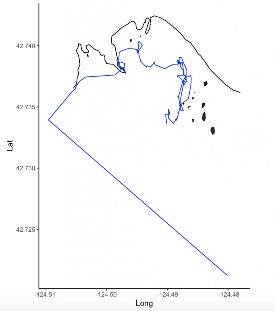
The first step in this process is to run a speed filter over each trackline. The aim of the speed filter is to remove any erroneous points or outliers that must be wrong based on the known travel speeds of gray whales. Barb Lagerquist, a Marine Mammal Institute (MMI) colleague who has tracked gray whales for several field seasons, found that the fastest individual she ever encountered traveled at a speed of 17.3 km/h (personal communication). Therefore, based on this information,  my tracklines are run through a speed filter set to remove any points that suggest that the whale traveled at 17.3 km/h or faster (Figure 2). 

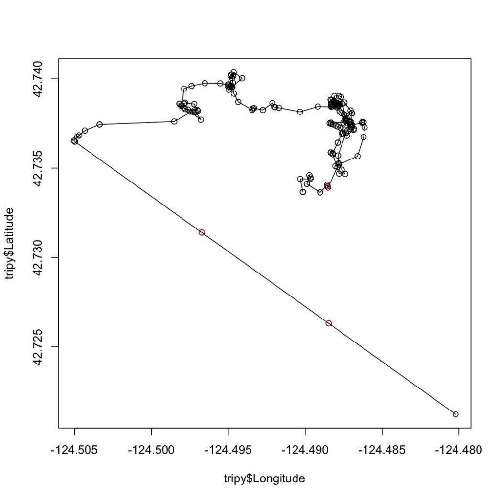
Fig 3. Trackline of “Humpy” after interpolation. The red points are interpolated.

Next, the speed-filtered tracklines are interpolated (Figure 3). Interpolation fills spatial and/or temporal gaps in a data set by evenly spacing points (by distance or time interval) between adjacent points. These gaps sometimes occur in my tracklines when the tracking teams misses one or several surfacings of a whale or because the whale is obscured by a large rock. 

After speed filtration and interpolation has occurred, the tracklines are ready to be analyzed using Residence in Space and Time (RST; Torres et al. 2017) to assign behavior state to each location. The questions I am hoping to answer for my thesis are based upon knowing the behavioral state of a whale at a given location and time. In order for me to draw conclusions over whether or not a whale prefers to forage by a reef with kelp rather than a reef without kelp, or whether it prefers Holmesimysis sculpta over Neomysis rayii, I need to know when a whale is actually foraging and when it is not. When we track whales from our cliff site, we assign a behavior to each marked location of an individual. It may sound simple to pick the behavior a whale is currently exhibiting, however it is much harder than it seems. Sometimes the behavioral state of a whale only becomes apparent after tracking it for several minutes. Yet, it’s difficult to change behaviors retroactively while tracking a whale and the qualitative assignment of behavior states is not an objective method. Here is where RST comes in.

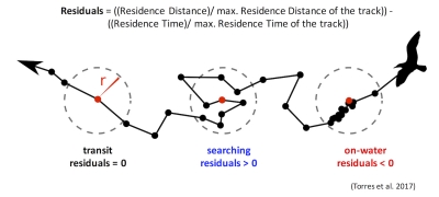
Those of you who have been following the blog for a few years may recall a post written in early 2017 by Rachael Orben, a former post-doc in the GEMM Lab who currently leads the Seabird Oceanography Lab. The post discussed the paper “Classification of Animal Movement Behavior through Residence in Space Time” written by Leigh and Rachael with two other collaborators, which had just been published a few days prior. If you want to know the nitty gritty of what RST is and how it works, I suggest reading Rachael’s blog, the GEMM lab’s brief description of the project and/or the actual paper since it is an open-access publication. However, in a nut shell, RST allows a user to identify three primary behavioral states in a tracking dataset based on the time and distance the individual spent within a given radius. The three behavioral categories are as follows:

Fig 4. Visualization of the three RST behavioral categories. Taken from Torres et al. (2017).
  • Transit – characterized by short time and distance spent within an area (radius of given size), meaning the individual is traveling.
  • Time-intensive – characterized by a long time spent within an area, meaning the individual is spending relatively more time but not moving much distance (such as resting in one spot). 
  • Time & distance-intensive – characterized by relatively high time and distances spent within an area, meaning the individual is staying within and moving around a lot in an area, such as searching or foraging. 

What behavior these three categories represent depends on the resolution of the data analyzed. Is one point every day for two years? Then the data are unlikely to represent resting. Or is the data 1 point every second for 1 hour? In which case travel segments may cover short distances. On average, my gray whale tracklines are composed of a point every 4-5 minutes for 1-2 hours.  Bases on this scale of tracking data, I will interpret the categories as follows: Transit is still travel, time & distance-intensive points represent locations where the whale was searching because it was moving around one area for a while, and time-intensive points represent foraging behavior because the whale has ‘found what it is looking for’ and is spending lots of time there but not moving around much anymore. The great thing about RST is that it removes the bias that is introduced by my field team when assigning behavioral states to individual whales (Figure 5). RST looks at the tracklines in a very objective way and determines the behavioral categories quantitatively, which helps to remove the human subjectivity.

While it took quite a bit of troubleshooting in R and overcoming error messages to make the codes run on my data, I am proud to have results that are interesting and meaningful with which I can now start to answer some of my many research questions. My next steps are to create interpolated prey density and distance to kelp layers in ArcGIS. I will then be able to overlay my cleaned up tracklines to start teasing out potential patterns and relationships between individual whale foraging movements and their environment. 

Literature cited

Torres, L. G., R. A. Orben, I. Tolkova, and D. R. Thompson. 2017. Classification of animal movement behavior through residence in space and time. PLoS ONE: doi. org/10.1371/journal.pone.0168513.

Demystifying the algorithm

By Clara Bird, Masters Student, OSU Department of Fisheries and Wildlife, Geospatial Ecology of Marine Megafauna Lab

Hi everyone! My name is Clara Bird and I am the newest graduate student in the GEMM lab. For my master’s thesis I will be using drone footage of gray whales to study their foraging ecology. I promise to talk about how cool gray whales in a following blog post, but for my first effort I am choosing to write about something that I have wanted to explain for a while: algorithms. As part of previous research projects, I developed a few semi-automated image analysis algorithms and I have always struggled with that jargon-filled phrase. I remember being intimidated by the term algorithm and thinking that I would never be able to develop one. So, for my first blog I thought that I would break down what goes into image analysis algorithms and demystify a term that is often thrown around but not well explained.

What is an algorithm?

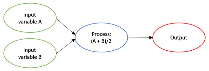
The dictionary broadly defines an algorithm as “a step-by-step procedure for solving a problem or accomplishing some end” (Merriam-Webster). Imagine an algorithm as a flow chart (Fig. 1), where each step is some process that is applied to the input(s) to get the desired output. In image analysis the output is usually isolated sections of the image that represent a specific feature; for example, isolating and counting the number of penguins in an image. Algorithm development involves figuring out which processes to use in order to consistently get desired results. I have conducted image analysis previously and these processes typically involve figuring out how to find a certain cutoff value. But, before I go too far down that road, let’s break down an image and the characteristics that are important for image analysis.

Figure 1. An example of a basic algorithm flow chart. There are two inputs: variables A and B. The process is the calculation of the mean of the two variables.

What is an image?

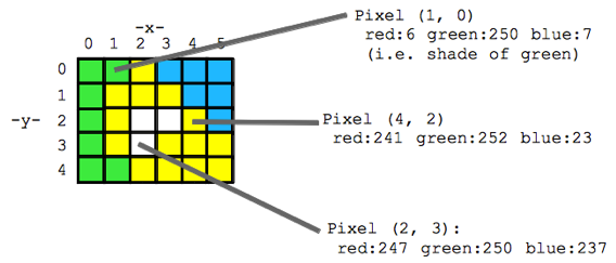
Think of an image as a spread sheet, where each cell is a pixel and each pixel is assigned a value (Fig. 2). Each value is associated with a color and when the sheet is zoomed out and viewed as a whole, the image comes together.  In color imagery, which is also referred to as RGB, each pixel is associated with the values of the three color bands (red, green, and blue) that make up that color. In a thermal image, each pixel’s value is a temperature value. Thinking about an image as a grid of values is helpful to understand the challenge of translating the larger patterns we see into something the computer can interpret. In image analysis this process can involve using the values of the pixels themselves or the relationships between the values of neighboring pixels.

Figure 2. A diagram illustrating how pixels make up an image. Each pixel is a grid cell associated with certain values. Image Source: https://web.stanford.edu/class/cs101/image-1-introduction.html

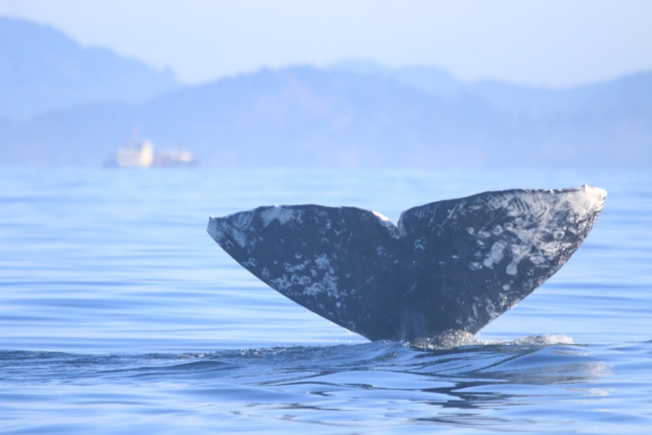
Our brains take in the whole picture at once and we are good at identifying the objects and patterns in an image. Take Figure 3 for example: an astute human eye and brain can isolate and identify all the different markings and scars on the fluke. Yet, this process would be very time consuming. The trick to building an algorithm to conduct this work is figuring out what processes or tools are needed to get a computer to recognize what is marking and what is not. This iterative process is the algorithm development.

Figure 3. Photo ID image of a gray whale fluke.

Development

An image analysis algorithm will typically involve some sort of thresholding. Thresholds are used to classify an image into groups of pixels that represent different characteristics. A threshold could be applied to the image in Figure 3 to separate the white color of the markings on the fluke from the darker colors in the rest of the image. However, this is an oversimplification, because while it would be pretty simple to examine the pixel values of this image and pick a threshold by hand, this threshold would not be applicable to other images. If a whale in another image is a lighter color or the image is brighter, the pixel values would be different enough from those in the previous image for the threshold to inaccurately classify the image. This problem is why a lot of image analysis algorithm development involves creating parameterized processes that can calculate the appropriate threshold for each image.

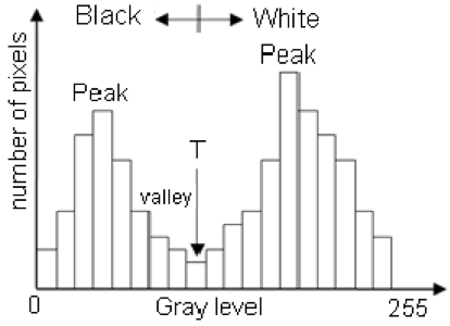
One successful method used to determine thresholds in images is to first calculate the frequency of color in each image, and then apply the appropriate threshold. Fletcher et al. (2009) developed a semiautomated algorithm to detect scars in seagrass beds from aerial imagery by applying an equation to a histogram of the values in each image to calculate the threshold. A histogram is a plot of the frequency of values binned into groups (Fig. 4). Essentially, it shows how many times each value appears in an image. This information can be used to define breaks between groups of values. If the image of the fluke were transformed to a gray scale, then the values of the marking pixels would be grouped around the value for white and the other pixels would group closer to black, similar to what is shown in Figure 4. An equation can be written that takes this frequency information and calculates where the break is between the groups. Since this method calculates an individualized threshold for each image, it’s a more reliable method for image analysis. Other characteristics could also be used to further filter the image, such as shape or area.

However, that approach is not the only way to make an algorithm applicable to different images; semi-automation can also be helpful. Semi-automation involves some kind of user input. After uploading the image for analysis, the user could also provide the threshold, or the user could crop the image so that only the important components were maintained. Keeping with the fluke example, the user could crop the image so that it was only of the fluke. This would help reduce the variety of colors in the image and make it easier to distinguish between dark whale and light marking.

Figure 4. Example histogram of pixel values. Source: Moallem et al. 2012

Why algorithms are important

Algorithms are helpful because they make our lives easier. While it would be possible for an analyst to identify and digitize each individual marking from a picture of a gray whale, it would be extremely time consuming and tedious. Image analysis algorithms significantly reduce the time it takes to process imagery. A semi-automated algorithm that I developed to count penguins from still drone imagery can count all the penguins on a one km2 island in about 30 minutes, while it took me 24 long hours to count them by hand (Bird et al. in prep). Furthermore, the process can be repeated with different imagery and analysts as part of a time series without bias because the algorithm eliminates human error introduced by different analysts.

Whether it’s a simple combination of a few processes or a complex series of equations, creating an algorithm requires breaking down a task to its most basic components. Development involves translating those components step by step into an automated process, which after many trials and errors, achieves the desired result. My first algorithm project took two years of revising, improving, and countless trials and errors.  So, whether creating an algorithm or working to understand one, don’t let the jargon nor the endless trials and errors stop you. Like most things in life, the key is to have patience and take it one step at a time.

References

Bird, C. N., Johnston, D.W., Dale, J. (in prep). Automated counting of Adelie penguins (Pygoscelis adeliae) on Avian and Torgersen Island off the Western Antarctic Peninsula using Thermal and Multispectral Imagery. Manuscript in preparation

Fletcher, R. S., Pulich, W. ‡, & Hardegree, B. (2009). A Semiautomated Approach for Monitoring Landscape Changes in Texas Seagrass Beds from Aerial Photography. https://doi.org/10.2112/07-0882.1

Moallem, Payman & Razmjooy, Navid. (2012). Optimal Threshold Computing in Automatic Image Thresholding using Adaptive Particle Swarm Optimization. Journal of Applied Research and Technology. 703.

Surveying for marine mammals in the Northern California Current

By Dawn Barlow, PhD student, OSU Department of Fisheries and Wildlife, Geospatial Ecology of Marine Megafauna Lab

There is something wonderful about time at sea, where your primary obligation is to observe the ocean from sunrise to sunset, day after day, scanning for signs of life. After hours of seemingly empty blue with only an occasional albatross gliding over the swells on broad wings, it is easy to question whether there is life in the expansive, blue, offshore desert. Splashes on the horizon catch your eye, and a group of dolphins rapidly approaches the ship in a flurry of activity. They play in the ship’s bow and wake, leaping out of the swells. Then, just as quickly as they came, they move on. Back to blue, for hours on end… until the next stirring on the horizon. A puff of exhaled air from a whale that first might seem like a whitecap or a smudge of sunscreen or salt spray on your sunglasses. It catches your eye again, and this time you see the dark body and distinctive dorsal fin of a humpback whale.

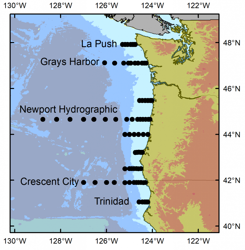
I have just returned from 10 days aboard the NOAA ship Bell M. Shimada, where I was the marine mammal observer on the Northern California Current (NCC) Cruise. These research cruises have sampled the NCC in the winter, spring, and fall for decades. As a result, a wealth of knowledge on the oceanography and plankton community in this dynamic ocean ecosystem has been assimilated by a dedicated team of scientists (find out more via the Newportal Blog). Members of the GEMM Lab have joined this research effort in the past two years, conducting marine mammal surveys during the transits between sampling stations (Fig. 2).

Figure 2. Northern California Current cruise sampling locations, where oceanography and plankton data are collected. Marine mammal surveys were conducted on the transits between stations.

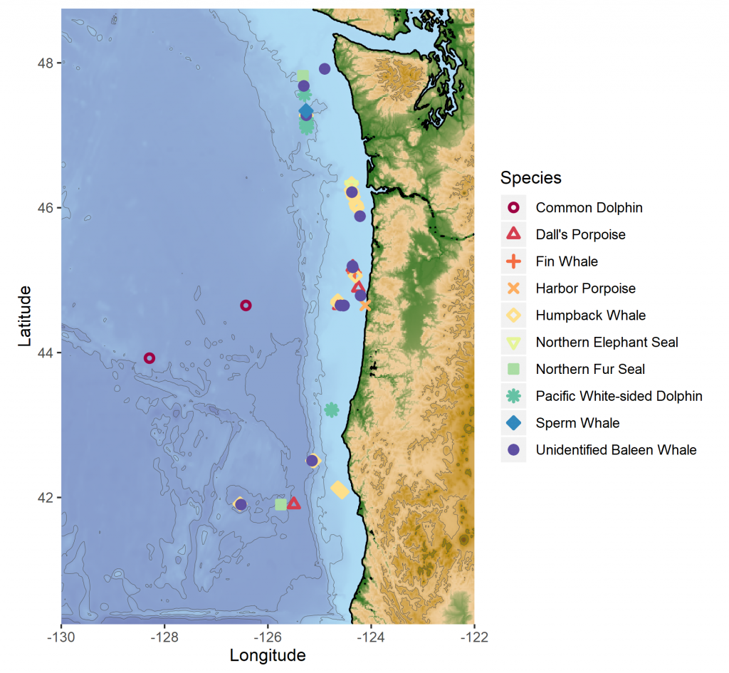
The fall 2019 NCC cruise was a resounding success. We were able to survey a large swath of the ecosystem between Crescent City, CA and La Push, WA, from inshore to 200 miles offshore. During that time, I observed nine different species of marine mammals (Table 1). As often as I use some version of the phrase “the marine environment is patchy and dynamic”, it never fails to sink in a little bit more every time I go to sea. On the map in Fig. 3, note how clustered the marine mammal sightings are. After nearly a full day of observing nothing but blue water, I would find myself scrambling to keep up with recording all the whales and dolphins we were suddenly in the midst of. What drives these clusters of sightings? What is it about the oceanography and prey community that makes any particular area a hotspot for marine mammals? We hope to get at these questions by utilizing the oceanographic data collected throughout the surveys to better understand environmental drivers of these distribution patterns.

 Table 1. Summary of marine mammal sightings from the September 2019 NCC Cruise.

Species # sightings Total # individuals
Northern Elephant Seal 1 1
Northern Fur Seal 2 2
Common Dolphin 2 8
Pacific White-sided Dolphin 8 143
Dall’s Porpoise 4 19
Harbor Porpoise 1 3
Sperm Whale 1 1
Fin Whale 1 1
Humpback Whale 22 36
Unidentified Baleen Whale 14 16
Figure 3. Map of marine mammal sighting locations from the September NCC cruise.

It was an auspicious time to survey the Northern California Current. Perhaps you have read recent news reports warning about the formation of another impending marine heatwave, much like the “warm blob” that plagued the North Pacific in 2015. We experienced it first-hand during the NCC cruise, with very warm surface waters off Newport extending out to 200 miles offshore (Fig. 4). A lot of energy input from strong winds would be required to mix that thick, warm layer and allow cool, nutrient-rich water to upwell along the coast. But it is already late September, and as the season shifts from summer to fall we are at the end of our typical upwelling season, and the north winds that would typically drive that mixing are less likely. Time will tell what is in store for the NCC ecosystem as we face the onset of another marine heatwave.

Figure 4. Temperature contours over the upper 150 m from 1-200 miles off Newport, Oregon from Fall 2014-2019. During Fall 2014, the Warm Blob inundated the Oregon shelf. Surface temperatures during that survey were 17°- 18°C along the entire transect. During 2015 and 2016 the warm water (16°C) layer had deepened and occupied the upper 50 m. During 2018, the temperature was 16°C in the upper 20 m and cooler on the shelf, indicative of residual upwelling. During this survey in 2019, we again saw very warm (18°C) temperatures in the upper water column over the entire transect. Image and caption credit: Jennifer Fisher.

It was a joy to spend 10 days at sea with this team of scientists. Insight, collaboration, and innovation are born from interdisciplinary efforts like the NCC cruises. Beyond science, what a privilege it is to be on the ocean with a group of people you can work with and laugh with, from the dock to 200 miles offshore, south to north and back again.

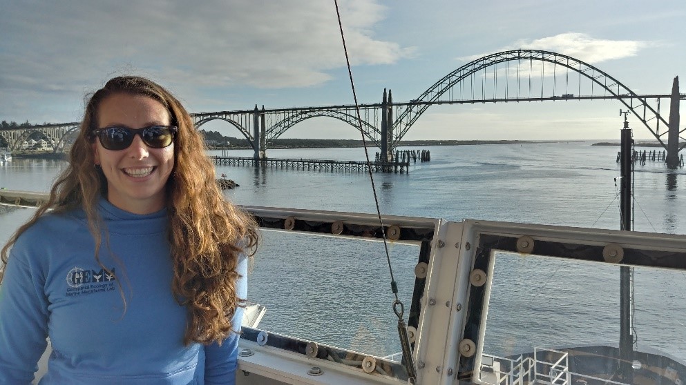
Dawn Barlow on the flying bridge of NOAA Ship Bell M. Shimada, heading out to sea with the Newport bridge in the background. Photo: Anna Bolm.