Maddie Honomichl, CSUMB Undergraduate in Marine Science, 2025 NSF REU and TOPAZ/JASPER Intern
Hi everyone, my name is Maddie Honomichl, and I was one of the two NSF REU interns with the GEMM lab this summer. This fall will be my last semester at California State University, Monterey Bay (CSUMB), where I will receive my undergraduate degree in Marine Science. Growing up in the Arizona desert limited my exposure to large bodies of water but led to memorable family trips to San Diego. With each trip my adoration for the ocean and the vast marine ecosystem emerged, resulting in my choice to go to college at CSU Monterey Bay. During my time at CSUMB, I learned of what internships were and the magnitude of impact these experiences had on my peers. Naturally, I searched online for weeks for future summer internship openings available—eventually leading me to none other than the GEMM Lab’s TOPAZ/JASPER project.
Celest Sorrentino, my amazing mentor, took me under her wing and helped me complete my very first research project: In sync? Studying blow synchrony in blue and gray whale mother-calf pairs using drone footage. The aim of my project is to understand more about calf development in gray and blue whales by investigating changes in mother-calf blow synchrony. But what is synchrony?
Synchrony can be defined as two individuals attempting to match each other’s behavior (Novotny & Bente 2022) and promote mimicry and learning. For example, humpback whales teaching their calves vocalizations and song patterns to communicate is an instance of synchrony and social learning (Anjara 2018). Another example of synchrony in wildlife is energetic transfer, where a whale calf will swim in alignment with its mother’s slipstream to expend less energy (Norris & Prescott 1961). Just like these behaviors, blow synchrony is a measure we can use in marine mammal mother-calf pairs to evaluate their relationship with each other.
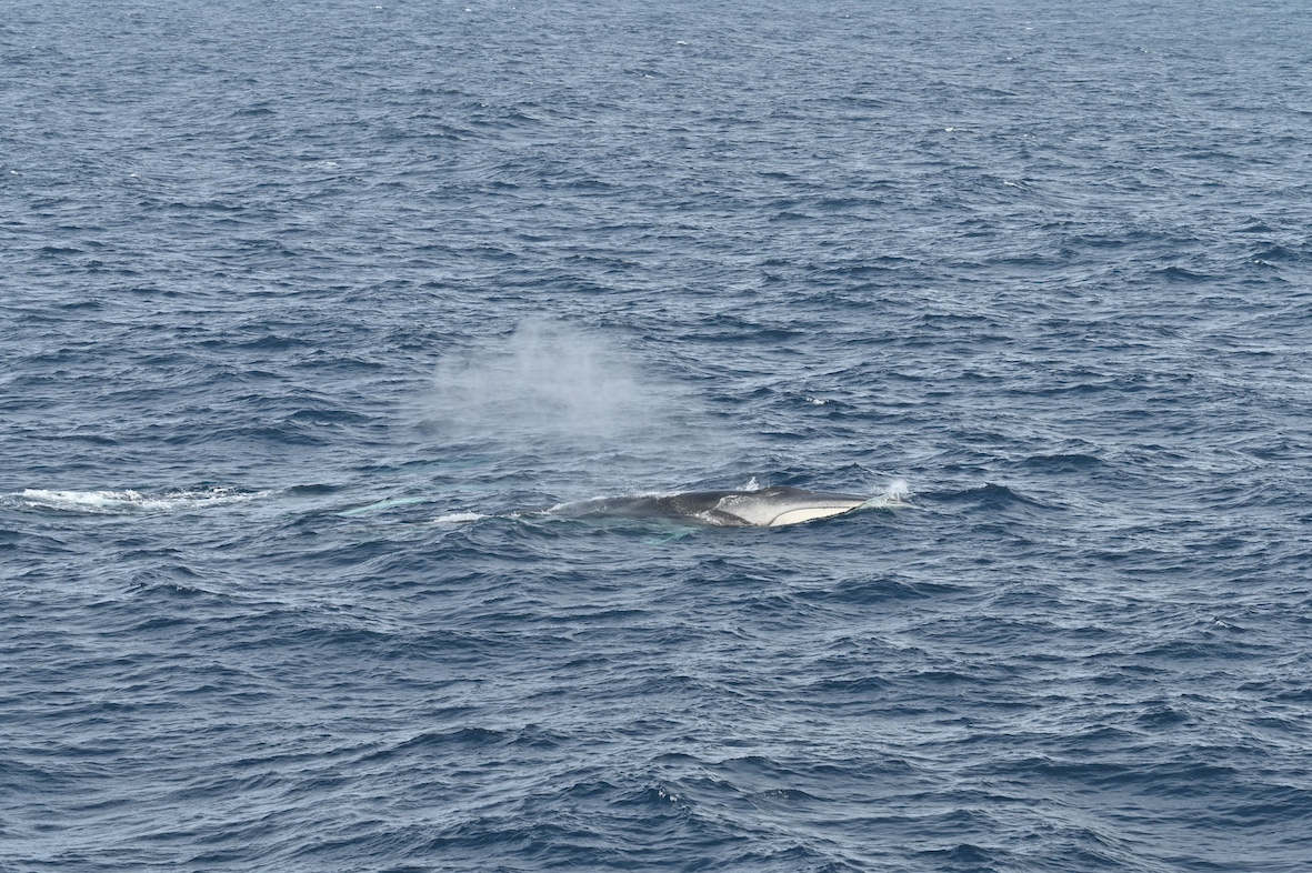
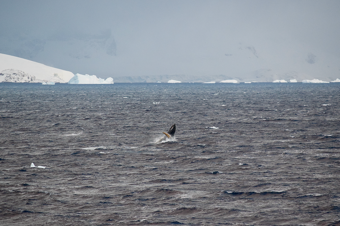
Aside from the TOPAZ/JASPER project, you might already be familiar with two other incredible GEMM lab projects GRANITE and SAPPHIRE. During the years of 2016-2023, drone footage of the Pacific Coast Feeding Group of gray whales was collected along the Oregon coast for the GRANITE project. In 2016, 2017, 2024, and 2025, drone footage for the pygmy blue whales was collected in South Taranaki Bight, New Zealand, for the SAPPHIRE project. Large marine mammals, especially whales, are difficult to study for many reasons including their brief occurrences at the surface and the challenges of studying aquatic animals. However, the use of drones allows for a safer and non-invasive alternative method for marine mammal monitoring in their natural habitat (Álvarez-González et al., 2023).
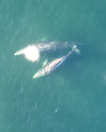
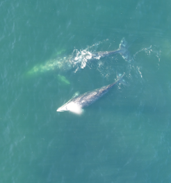
Figure 2. Two still images taken from GRANITE drone footage. The left is of a mother gray whale blowing and the right is of a gray whale calf blowing
Baleen whale calves only have 6-8 months to learn everything they need to know before they wean and are sent off on their own (Lockyer 1984). I don’t know about you, but if my mom kicked me out after I turned 5 years old, I would be pretty lost. In American culture, the golden age for humans to be considered an adult is around 18 years old, when they finally leave the house and venture on their own. For humans, age is a cultural sign of independence, but not much is known about what factors influence what makes a calf ready to be independent. Blow synchrony between mother-calf pairs during the calf’s weaning period can be used as a metric for calf development, which is important to know more about as calf development and survival rates are critical factors to consider in population dynamics and management efforts.
When do whales eventually leave their mother? We frequently don’t know how old a calf is, so we use three different metrics as proxies of calf maturity. First, we use Total Length (TL), which is the length of the whale from rostrum to fluke (or nose to tail) (Pirotta et. al., 2023) and serves as an indicator of growth. Our next metric is Body Area Index (BAI), similar to BMI in humans, which is a score of body condition to understand how fat or skinny the whale calf is (Burnett et. al., 2019). Total Length and BAI measurements are derived from drone photogrammetry work conducted by the GEMM Lab and CODEX. Our last proxy is Day of Year (DOY), which is the day in the year we sighted the whales.

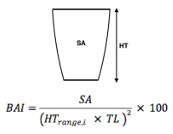
Figure 3. Demonstrating photogrammetry methods used to measure Total Length and Body Area Index (BAI). On the left is a drone image of a gray whale showing how we calculate Total Length (TL) from rostrum to fluke. This image is also divided into increments which are used to calculate Surface Area (SA), depicted by the green dashed box, and using the equation on the right with TL, BAI is calculated.
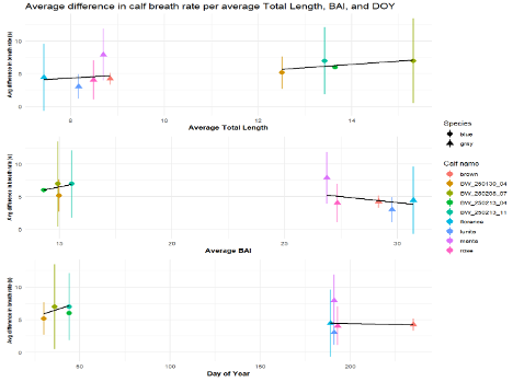
The specific question I addressed was: Does mother-calf blow rate synchrony change as the calf’s Total Length and Body Area Index increase, and Day of Year increases? In other words, does synchrony change as calves become longer, healthier, and the year progresses. Meaning, as the calf grows in length, increases its body condition, and the day of year progresses, the calf will gain independence from its mother and become out of sync.
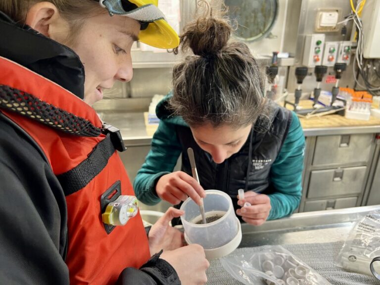
I analyzed blowhole rates of mother-calf gray and blue whales using a program called BORIS (Friard & Gamba 2016). BORIS (Behavioral Observation Research Interactive Software) is an online free program where researchers can assign behavior states to animals in video. In BORIS, I watched the drone footage and marked a “blow” event for the mom and calf, recording a specific time stamp per event. I repeated this workflow for each video of both gray and blue whale mom-calf pairs. Once completed, I calculated the average difference of the calf’s timestamp from the mother’s timestamp per pair. The reason behind this approach is that the larger the average difference, the more asynchronous the calf is with its mother, and the smaller the average difference the more synchronous they will become.
To evaluate the effect of our proxies for age, Total Length, BAI, and Day of Year, on mother-calf blow rate synchrony, I turned to my good friend RStudio. I created a scatterplot and regressions for these relationships (Figure 4). These results indicate that body condition (BAI) may be a better proxy of calf maturity and preparation for weaning in gray whales (p-value = 0.0064), whereas calf Total Length (TL) is more indicative of calf maturity in blue whales (p-value = 0.00097).
As I end my 10-week internship summer filled with data collection and analysis, lots of laughs and inside jokes, I am proud to say I have learned so much about the research that goes into a project like mine. As someone who loves marine animals, especially whale sharks, I now have a newfound love for whales that will forever be in my heart. I am so incredibly grateful that I was able to work with the GEMM lab and the amazing team of researchers and scientists it encompasses. Being a first-generation college student comes with its challenges of learning how to navigate higher education without direct guidance of family who had been through the experience. But if there’s one thing I always tell myself, it’s that with a little bit of grit and hard work, you can do anything you put your mind to! Whatever my future holds for me, I hope it is filled with more research opportunities and the chance to work with marine mammals!
References:
Álvarez-González, M., Suarez-Bregua, P., Pierce, G. J., & Saavedra, C. (2023). Unmanned Aerial Vehicles (UAVs) in Marine Mammal Research: A Review of Current Applications and Challenges. Drones, 7(11), 667. https://doi.org/10.3390/drones7110667
Anjara Saloma. Humpback whales (Megaptera novaeangliae) mother-calf interactions. Vertebrate Zoology. Université Paris Saclay (COmUE); Université d’Antananarivo, 2018. English. ⟨NNT : 2018SACLS138⟩. ⟨tel-02869389⟩
Burnett, J. D., Lemos, L., Barlow, D., Wing, M. G., Chandler, T., & Torres, L. G. (2019). Estimating morphometric attributes of baleen whales with photogrammetry from small UASs: A case study with blue and gray whales. Marine Mammal Science, 35(1), 108–139. https://doi.org/10.1111/mms.12527
Friard, O., & Gamba, M. (2016). BORIS: A free, versatile open‐source event‐logging software for video/audio coding and live observations. Methods in Ecology and Evolution, 7(11), 1325–1330. https://doi.org/10.1111/2041-210X.12584
Huetz, C., Saloma, A., Adam, O., Andrianarimisa, A., & Charrier, I. (2022). Ontogeny and synchrony of diving behavior in Humpback whale mothers and calves on their breeding ground. Journal of Mammalogy, 103(3), 576–585. https://doi.org/10.1093/jmammal/gyac010
Lockyer, Christina. (1984). Review of Baleen Whale (Mysticeti) Reproduction and Implications for Management. Reproduction in whales, dolphins and porpoises. Proc. conference, La Jolla, CA, 1981. 6. 27-50.
Norris, K.S., & Prescott, J.H. (1961). Observations of Pacific cetaceans of Californian and Mexican waters. University of California Publications in Zoology, 63, 291- 402.
Novotny, E., & Bente, G. (2022). Identifying Signatures of Perceived Interpersonal Synchrony. Journal of nonverbal behavior, 46(4), 485–517. https://doi.org/10.1007/s10919-022-00410-9
Pirotta, E., Fernandez Ajó, A., Bierlich, K. C., Bird, C. N., Buck, C. L., Haver, S. M., Haxel, J. H., Hildebrand, L., Hunt, K. E., Lemos, L. S., New, L., & Torres, L. G. (2023). Assessing variation in faecal glucocorticoid co
Smultea, M. A., Fertl, D., Bacon, C. E., Moore, M. R., James, V. R., & Würsig, B. (2017). Cetacean mother-calf behavior observed from a small aircraft off Southern California. Animal Behavior and Cognition, 4(1), 1–23. https://doi.org/10.12966/abc.01.02.2017