By Dr. Dawn Barlow, Postdoctoral Scholar, OSU Department of Fisheries, Wildlife, and Conservation Sciences, Geospatial Ecology of Marine Megafauna Lab
Imagine you are 50 nautical miles from shore, perched on the observation platform of a research vessel. The ocean is blue, calm, and seems—for all intents and purposes—empty. No birds fly overhead, nothing disturbs the rolling swells except the occasional whitecap from a light breeze. The view through your binoculars is excellent, and in the distance, you spot a disturbance at the surface of the water. As the ship gets closer, you see splashing, and a flurry of activity emerges as a large group of dolphins leap and dive, likely chasing a school of fish. They swim along with the ship, riding the bow-wave in a brief break from their activity. Birds circle in the air above them and float on the water around them. Together with your team of observers, you rush to record the species, the number of animals, their distance to the ship, and their behavior. The research vessel carries along its pre-determined trackline, and the feeding frenzy of birds and dolphins fades off behind you as quickly as it came. You return to scanning the blue water.

The marine environment is highly dynamic, and resources in the ocean are notoriously patchy. One of our main objectives in marine ecology is to understand what drives these ephemeral hotspots of species diversity and biological activity. This objective is particularly important now as the oceans warm and shift. In the context of rapid global climate change, there is a push to establish alternatives to fossil fuels that can support society’s energy needs while minimizing the carbon emissions that are a root cause of climate change. One emergent option is offshore wind, which has become a hot topic on the West Coast of the United States in recent years. The technology has the potential to supply a clean energy source, but the infrastructure could have environmental and societal impacts of its own, depending on where it is placed, how it is implemented, and when it is operational.

Any development in the marine environment, including alternative energy such as offshore wind, should be undertaken using the best available scientific knowledge of the ecosystem where it will be implemented. The Marine Mammal Institute’s collaborative project, Marine Offshore Species Assessments to Inform Clean energy (MOSAIC), was designed for just this reason. As the name “MOSAIC” implies, it is all about using different tools to compile different datasets to establish crucial baseline information on where marine mammals and seabirds are distributed in Oregon and Northern California, a region of interest for wind energy development.
A MOSAIC of species
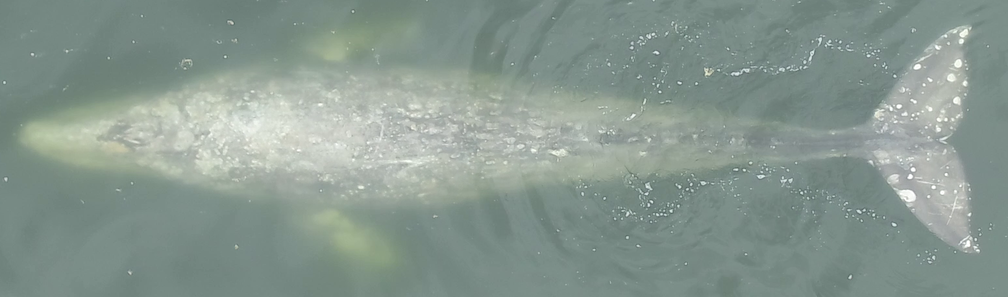
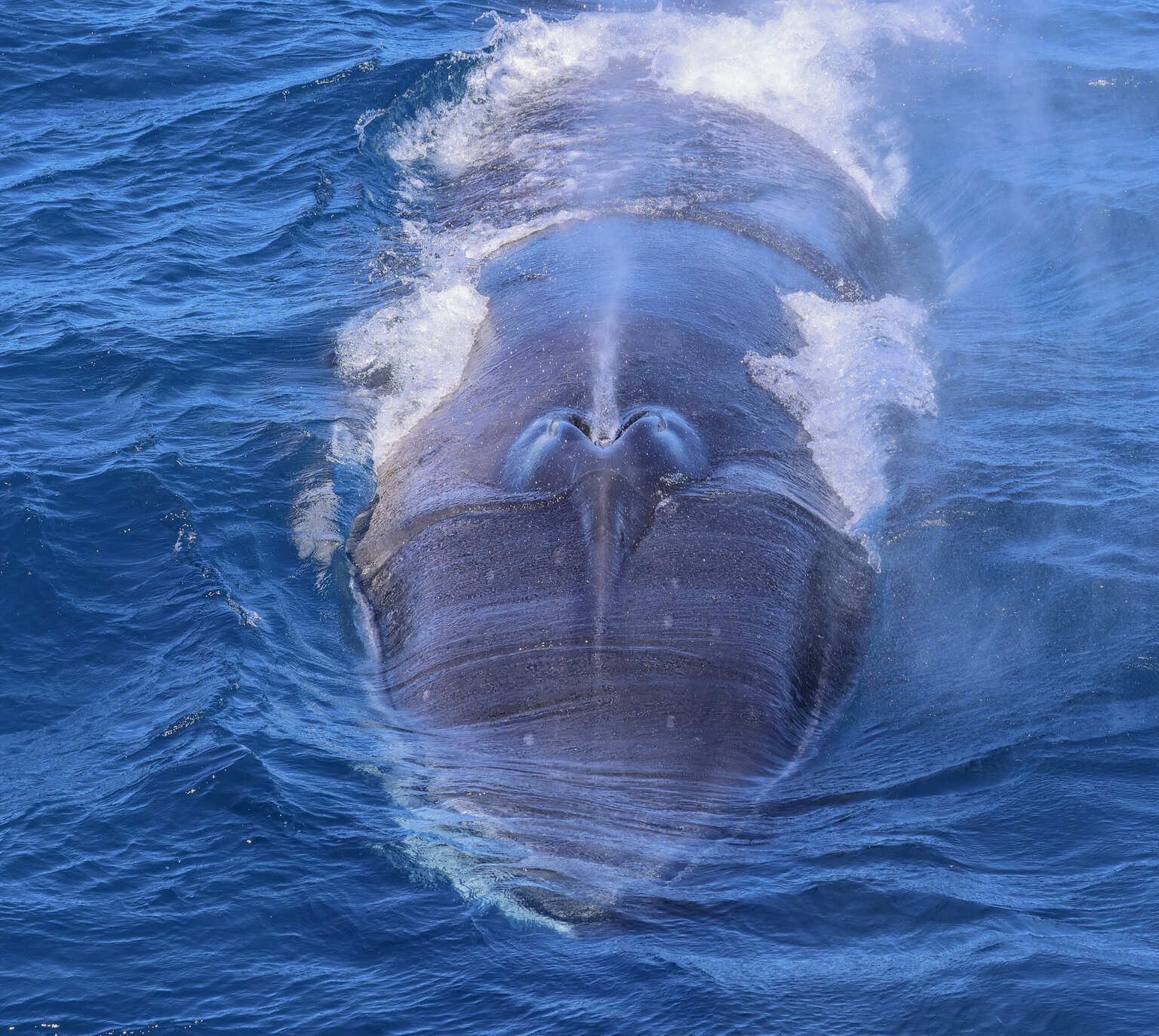
The waters of Oregon and Northern California are rich with life. Numerous cetaceans are found here, from the largest species to ever live, the blue whale, to one of the smallest cetaceans, the harbor porpoise, with many species filling in the size range in between: fin whales, humpback whales, sperm whales, killer whales, Risso’s dolphins, Pacific white-sided dolphins, northern right whale dolphins, and Dall’s porpoises, to name a few. Seabirds likewise rely on these productive waters, from the large, graceful albatrosses that feature in maritime legends, to charismatic tufted puffins, to the little Leach’s storm petrels that could fit in the palm of your hand yet cover vast distances at sea. From our data collection efforts so far, we have already documented 16 cetacean species and 64 seabird species.

A MOSAIC of data and tools

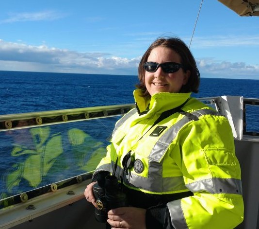
Through the four-year MOSAIC project, we are undertaking two years of visual surveys and passive acoustic monitoring from Cape Mendocino to the mouth of the Columbia River on the border of Oregon and Washington and seaward to the continental slope. Six comprehensive surveys for cetaceans and seabirds are being conducted aboard the R/V Pacific Storm following a carefully chosen trackline to cover a variety of habitats, including areas of interest to wind energy developers.
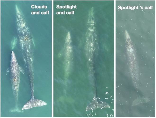
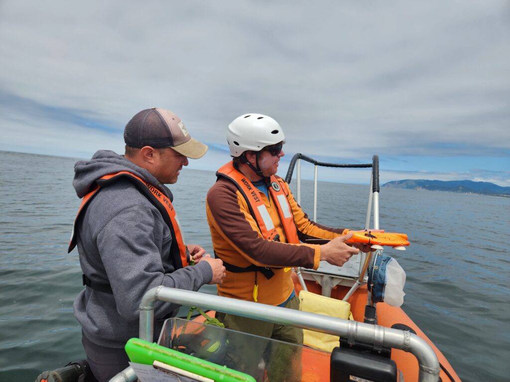
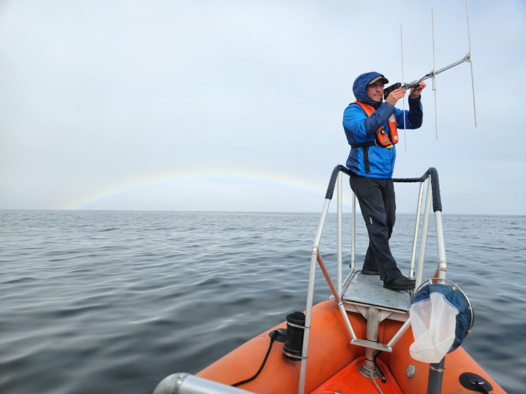
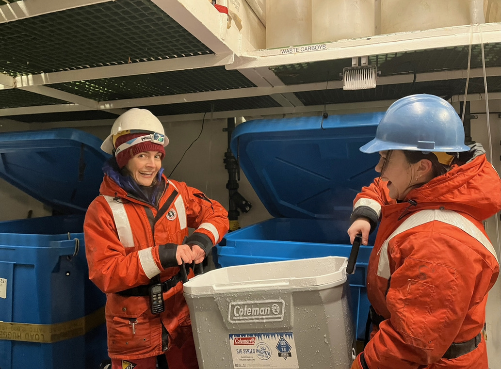
These dedicated surveys are complemented by additional surveys conducted aboard NOAA research vessels during collaborative expeditions in the Northern California Current, and ongoing aerial surveys in partnership with the United States Coast Guard through the GEMM Lab’s OPAL project. Three bottom-mounted hydrophones were deployed in August 2022, and are recording cetacean vocalizations and the ambient soundscape, and these recordings will be complemented by acoustic data that is being collected continuously by the Oceans Observing Initiative. In addition to these methods to collect broad-scale species distribution information, concurrent efforts are being conducted via small boats to collect individual identification photographs of baleen whales and tissue biopsy samples for genetic analysis. Building on the legacy of satellite tracking here at the Marine Mammal Institute, the MOSAIC project is breathing new life into tag data from large whales to assess movement patterns over many years and determine the amount of time spent within our study area.

The resulting species occurrence data from visual surveys and acoustic monitoring will be integrated to develop Species Distribution Models for the many different species in our study region. Identification photographs of individual baleen whales, DNA profiles from whale biopsy samples, and data from satellite-tagged whales will provide detailed insight into whale population structure, behavior, and site fidelity (i.e., how long they typically stay in a given area), which will add important context to the distribution data we collect through the visual surveys and acoustic monitoring. The models will be implemented to produce maps of predicted species occurrence patterns, describing when and where we expect different cetaceans and seabirds to be under different environmental conditions.
With five visual surveys down, the MOSAIC team is gearing up for one final survey this month. The hydrophones will be retrieved this summer. Then, with data in-hand, the team will dive deep into analysis.
A MOSAIC of collaborators

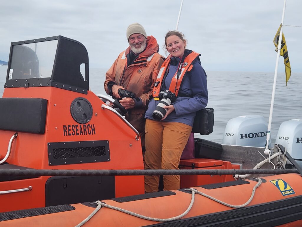
The collaborative MOSAIC team brings together a diverse set of tools. The depth of expertise here at the Marine Mammal Institute spans a broad range of disciplines, well-positioned to provide robust scientific knowledge needed to inform alternative energy development in Oregon and Northern California waters.
I have had the pleasure of participating in three of the six surveys aboard the R/V Pacific Storm, including leading one as Chief Scientist, and have collected visual survey data aboard NOAA Ship Bell M. Shimada and from United States Coast Guard helicopters over the years that will be incorporated in the MOSAIC of datasets for the project. This ecosystem is one that I feel deeply connected to from time spent in the field. Now, I am thrilled to dive into the analysis, and will lead the modeling of the visual survey data and the integration of the different components to produce species distribution maps for cetaceans and seabirds our study region.
This project is funded by the United States Department of Energy. The Principal Investigator is the Institute’s Director Dr. Lisa Ballance, and Co-Principal Investigators include Scott Baker, Barbara Lagerquist, Rachael Orben, Daniel Palacios, Kate Stafford, and Leigh Torres of the Marine Mammal Institute; John Calambokidis of the Cascadia Research Collective; and Elizabeth Becker of ManTech International Corp. For more information, please visit the project website, and stay tuned for updates as we enter the analysis phase.
Did you enjoy this blog? Want to learn more about marine life, research, and conservation? Subscribe to our blog and get a weekly alert when we make a new post! Just add your name into the subscribe box below!