By Amanda Rose Kent, College of Earth Ocean and Atmospheric Sciences, OSU, GEMM Lab/Krill Seeker undergraduate intern
If you asked me five years ago where I’d thought I’d be today, the answer I would give would not reflect where I am now. Back then, I was a customer service representative for a hazardous waste company, and I believed that going to university and participating in research was a straightforward experience. I learned soon after I left that career and began my journey at OSU in 2020 that I wasn’t even remotely aware of the process. I knew that as part of my oceanography degree I would need to become involved in some form of research, but I had no idea where to start.
I started looking through the Oregon State website and I eventually found an outdated flier from 2018 that advertised a lab that studied plankton in Antarctica, and that was when I first reached out to Dr. Kim Bernard. My journey took off from there. As an undergraduate researcher in the URSA Engage program working with Kim and one of her graduate students, Rachel, I conducted a literature review on the ecosystem services provided by two species of krill off the coast of Oregon, including their value to baleen whales. After learning all I could from the literature about krill and how important they were to the ocean, I knew that there was so much more to learn and that this was the topic I wanted to continue to pursue. After I completed the URSA program, I remained a member of Kim’s zooplankton ecology lab.
While continuing to work with Rachel, I was given the opportunity to join the GEMM Lab’s Project HALO for a daylong cruise conducting a whale survey along the Newport Hydrographic Line. I was initially brought on to learn how to use the echosounder to collect krill data but unfortunately, the device had technical difficulties and Rachel and I were no longer needed. We decided to go on the cruise anyway, and I was able to instead learn how to survey for marine mammals (it’s not as easy as it may seem, but still very fun!).
Figure 1. Enjoying the point of view from the crow’s nest on the R/V Pacific Storm, but also very cold.
Soon, another opportunity arose to apply for a brand-new program called ARC-Learn. This two-year research program focuses on studying the Arctic using publicly available data, and with the support of my mentors, I applied and was accepted. Initially I found that there were no mentors within the program that studied krill, so I found myself becoming immersed in a new topic: harmful algal blooms (HABs). Determined to incorporate krill into this research, I started looking through the literature trying to develop my hypothesis that HABs affected zooplankton in some way. There was evidence to potentially support my hypothesis, but I ended up encountering numerous data gaps in the region I was studying. After months of roadblocks, I eventually started feeling defeated and regretted applying for the program. Rachel was quick to remind me that all experiences are valuable experiences, and that I was still gaining new skills I could use in graduate school or my career.
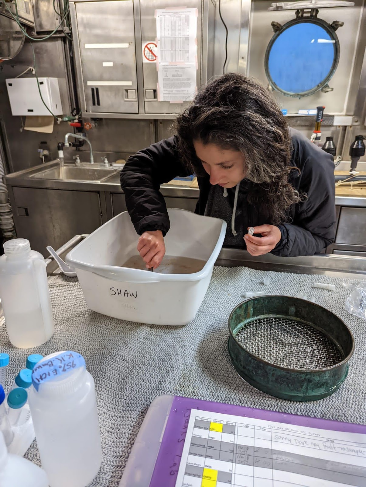
As my undergraduate degree progressed, I continued supporting Rachel in her graduate research, spending some time during the summer processing krill samples by sorting, sexing, and drying them to crush them into pellets. Our goal was to process them in an instrument called a bomb calorimeter, which is used to quantify the caloric content of prey species and help us better understand the energy flux required for animals higher up the food chain (like whales) and the amount they need to eat. I was only able to do this for a few weeks before heading out on the experience of a lifetime, spending three weeks on a ship traveling around the Bering, Chukchi, and Beaufort Seas with one of my ARC-Learn mentors. It was a great opportunity for me to see the toxic phytoplankton (which can form HABs) I had been studying and learn about methods of sample collection and processing. If I could go back and do it again, I’d go in a heartbeat.
Figure 2. Pulling out all of the animal biomass out of the Arctic sediment.
At the beginning of my bachelor’s degree, I had expected to just work with Kim and conduct research within her lab. Instead, I have had opportunities I would never have expected five years ago. I have learned a vast amount from my graduate mentor, Rachel, which has helped influence my trajectory in my degree. I have had the privilege to not only meet giants in the field I’m interested in, but also work with them and learn from them, and to spend three weeks in the Arctic Ocean. The experiences I have had throughout this roller-coaster helped me develop a project idea with new mentors that I eventually hope to pursue in my master’s degree. I wasn’t prepared for the number of adjustments I would make to find new experiences and start new projects, but all the experiences I had were necessary to learn about what I was interested in and what I wanted to pursue. Looking back on it all today, I have zero regrets.
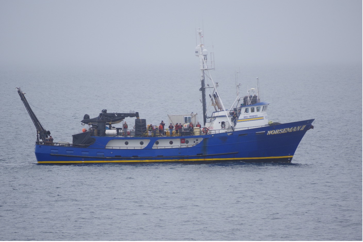
Figure 3. A picture of the Norseman II, the ship I was on in the Arctic, taken by the Japanese ship JAMSTEC on a short rendezvous between the Chukchi and Beaufort Seas.
1PhD student, Oregon State University College of Earth, Ocean, and Atmospheric Sciences and Department of Fisheries, Wildlife, and Conservation Sciences, Geospatial Ecology of Marine Megafauna Lab
What do peanut butter m&ms, killer whales, affogatos, tired eyes, and puffins all have in common? They were all major features of the recent Northern California Current (NCC) ecosystem survey cruise.
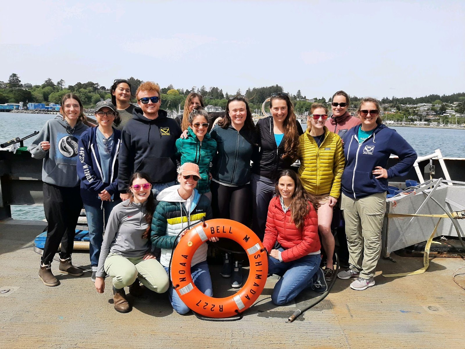
The science party of the May 2022 Northern California Current ecosystem cruise.
We spent May 6–17 aboard the NOAA vessel Bell M. Shimada in northern California, Oregon, and Washington waters. This fabulously interdisciplinary cruise studies multiple aspects of the NCC ecosystem three times per year, and the GEMM lab has put marine mammal observers aboard since 2018.
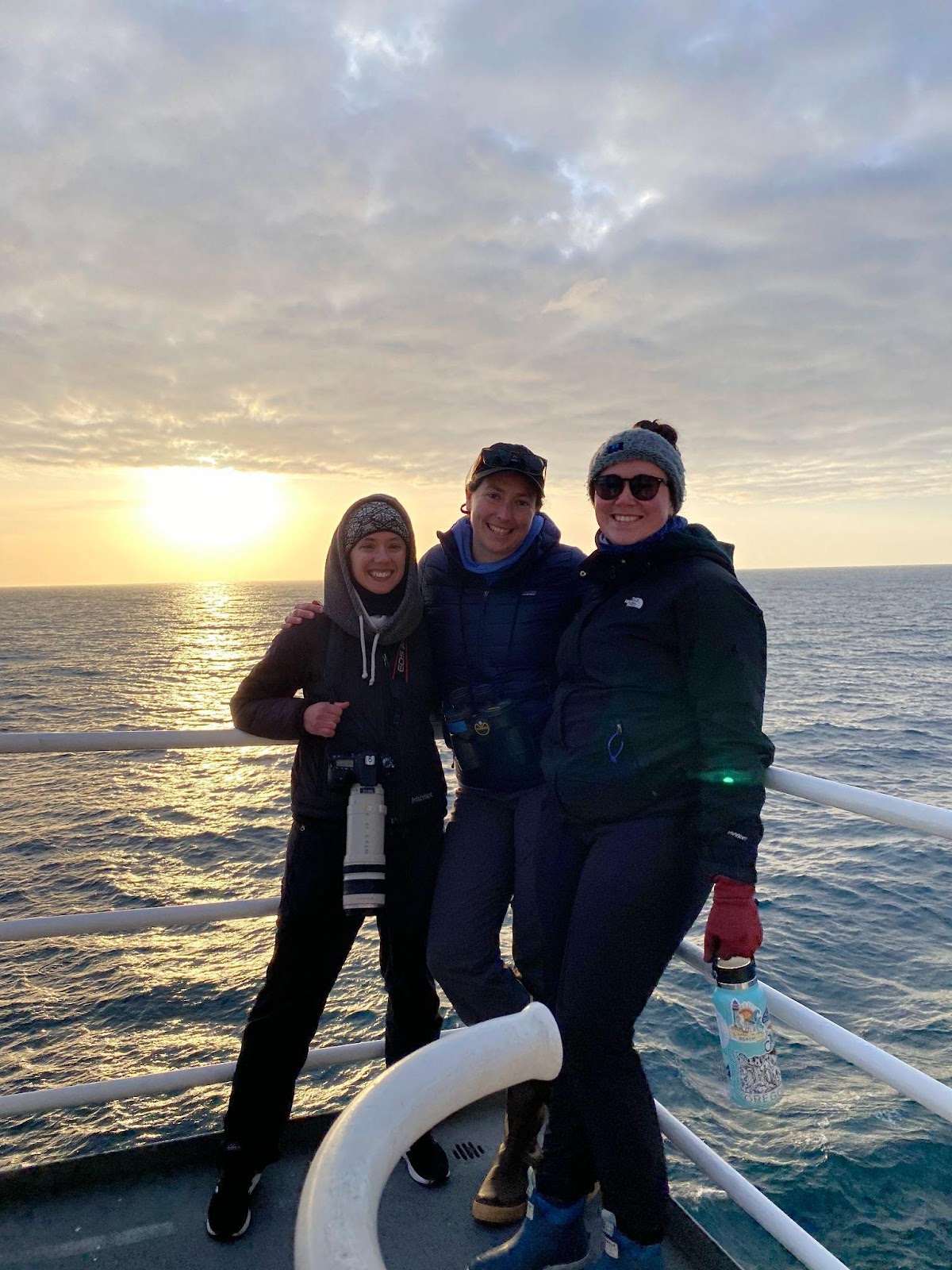
This cruise was a bit different than usual for the GEMM lab: we had eyes on both the whales and their prey. While Dawn Barlow and Clara Bird observed from sunrise to sunset to sight and identify whales, Rachel Kaplan collected krill data via an echosounder and samples from net tows in order to learn about the preyscape the whales were experiencing.
From left, Rachel, Dawn, and Clara after enjoying some beautiful sunset sightings.
We sailed out of Richmond, California and went north, sampling as far north as La Push, Washington and up to 200 miles offshore. Despite several days of challenging conditions due to wind, rain, fog, and swell, the team conducted a successful marine mammal survey. When poor weather prevented work, we turned to our favorite hobbies of coding and snacking.
Rachel attends “Clara’s Beanbag Coding Academy”.
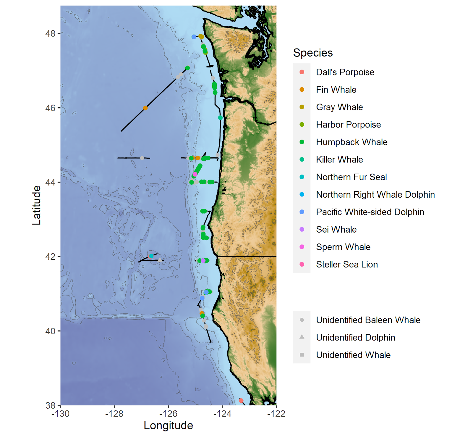
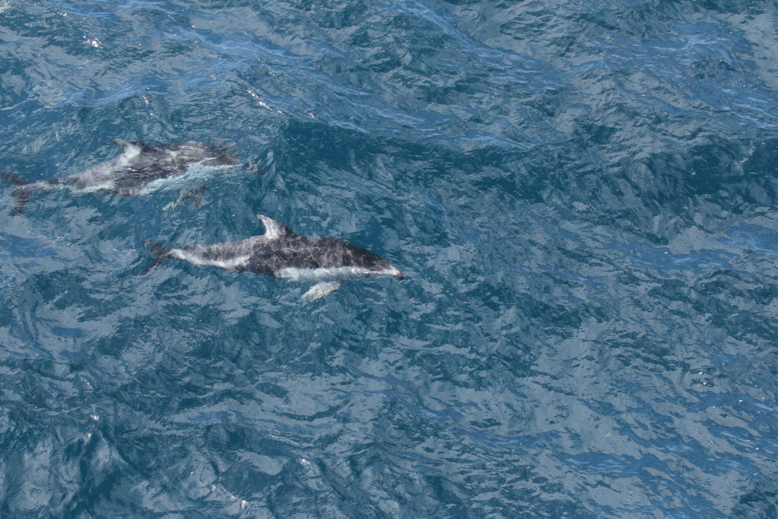
Cruise highlights included several fin whales, sperm whales, killer whales, foraging gray whales, fluke slapping and breaching humpbacks, and a visit by 60 pacific white-sided dolphins. While being stopped at an oceanographic sampling station typically means that we take a break from observing, having more time to watch the whales around us turned out to be quite fortunate on this cruise. We were able to identify two unidentified whales as sei whales after watching them swim near us while paused on station.
Marine mammal observation segments (black lines) and the sighting locations of marine mammal species observed during the cruise.
On one of our first survey days we also observed humpbacks surface lunge feeding close to the ship, which provided a valuable opportunity for our team to think about how to best collect concurrent prey and whale data. The opportunity to hone in on this predator-prey relationship presented itself in a new way when Dawn and Clara observed many apparently foraging humpbacks on the edge of Heceta Bank. At the same time, Rachel started observing concurrent prey aggregations on the echosounder. After a quick conversation with the chief scientist and the officers on the bridge, the ship turned around so that we could conduct a net tow in order to get a closer look at what exactly the whales were eating.
Success! Rachel collects krill samples collected in an area of foraging humpback whales.
This cruise captured an interesting moment in time: southerly winds were surprisingly common for this time of year, and the composition of the phytoplankton and zooplankton communities indicated that the seasonal process of upwelling had not yet been initiated. Upwelling brings deep, cold, nutrient-rich waters to the surface, generating a jolt of productivity that brings the ecosystem from winter into spring. It was fascinating to talk to all the other researchers on the ship about what they were seeing, and learn about the ways in which it was different from what they expected to see in May.
Experiencing these different conditions in the Northern California Current has given us a new perspective on an ecosystem that we’ve been observing and studying for years. We’re looking forward to digging into the data and seeing how it can help us understand this ecosystem more deeply, especially during a period of continued climate change.
The total number of each marine mammal species observed during the cruise.
Did you enjoy this blog? Want to learn more about marine life, research, and conservation? Subscribe to our blog and get a weekly message when we post a new blog. Just add your nameand email into the subscribe box below.
Dr. KC Bierlich, Postdoctoral Scholar, OSU Department of Fisheries, Wildlife, & Conservation Sciences, Geospatial Ecology of Marine Megafauna (GEMM) Lab
In a previous blog, I discussed the importance of incorporating measurement uncertainty in drone-based photogrammetry, as drones with different sensors, focal length lenses, and altimeters will have varying levels of measurement accuracy. In my last blog, I discussed how to incorporate photogrammetric uncertainty when combining multiple measurements to estimate body condition of baleen whales. In this blog, I will highlight our recent publication in Frontiers in Marine Science (https://doi.org/10.3389/fmars.2022.867258) led by GEMM Lab’s Dr. Leigh Torres, Clara Bird, and myself that used these methods in a collaborative study using imagery from four different drones to compare gray whale body condition on their breeding and feeding grounds (Torres et al., 2022).
Most Eastern North Pacific (ENP) gray whales migrate to their summer foraging grounds in Alaska and the Arctic, where they target benthic amphipods as prey. A subgroup of gray whales (~230 individuals) called the Pacific Coast Feeding Group (PCFG), instead truncates their migration and forages along the coastal habitats between Northern California and British Columbia, Canada (Fig. 1). Evidence from a recent study lead by GEMM Lab’s Lisa Hildebrand (see this blog) found that the caloric content of prey in the PCFG range is of equal or higher value than the main amphipod prey in the Arctic/sub-Arctic regions (Hildebrand et al., 2021). This implies that greater prey density and/or lower energetic costs of foraging in the Arctic/sub-Arctic may explain the greater number of whales foraging in that region compared to the PCFG range. Both groups of gray whales spend the winter months on their breeding and calving grounds in Baja California, Mexico.
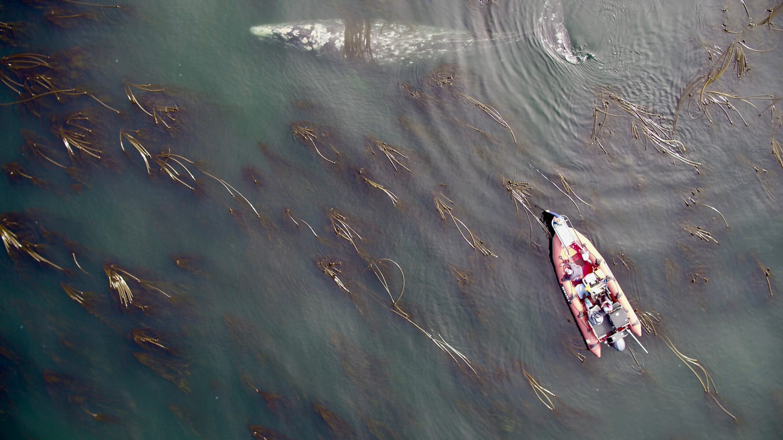
Figure 1. The GEMM Lab field team following a Pacific Coast Feeding Group (PCFG) gray whale swimming in a kelp bed along the Oregon Coast during the summer foraging season.
In January 2019 an Unusual Mortality Event (UME) was declared for gray whales due to the elevated numbers of stranded gray whales between Mexico and the Arctic regions of Alaska. Most of the stranded whales were emaciated, indicating that reduced nutrition and starvation may have been the causal factor of death. It is estimated that the population dropped from ~27,000 individuals in 2016 to ~21,000 in 2020 (Stewart & Weller, 2021).
During this UME period, between 2017-2019, the GEMM Lab was using drones to monitor the body condition of PCFG gray whales on their Oregon coastal feeding grounds (Fig. 1), while Christiansen and colleagues (2020) was using drones to monitor gray whales on their breeding grounds in San Ignacio Lagoon (SIL) in Baja California, Mexico. We teamed up with Christiansen and colleagues to compare the body condition of gray whales in these two different areas leading up to the UME. Comparing the body condition between these two populations could help inform which population was most effected by the UME.
The combined datasets consisted of four different drones used, thus different levels of photogrammetric uncertainty to consider. The GEMM Lab collected data using a DJI Phantom 3 Pro, DJI Phantom 4, and DJI Phantom 4 Pro, while Christiansen et al., (2020) used a DJI Inspire 1 Pro. By using the methodological approach described in my previous blog (here, also see Bierlich et al., 2021a for more details), we quantified photogrammetric uncertainty specific to each drone, allowing cross-comparison between these datasets. We also used Body Area Index (BAI), which is a standardized relative measure of body condition developed by the GEMM Lab (Burnett et al., 2018) that has low uncertainty with high precision, making it easier to detect smaller changes between individuals (see blog here, Bierlich et al., 2021b).
While both PCFG and ENP gray whales visit San Ignacio Lagoon in the winter, we assume that the photogrammetry data collected in the lagoon is mostly of ENP whales based on their considerably higher population abundance. We also assume that gray whales incur low energetic cost during migration, as gray whale oxygen consumption rates and derived metabolic rates are much lower during migration than on foraging grounds (Sumich, 1983).
Interestingly, we found that gray whale body condition on their wintering grounds in San Ignacio Lagoon deteriorated across the study years leading up to the UME (2017-2019), while the body condition of PCFG whales on their foraging grounds in Oregon concurrently increased. These contrasting trajectories in body condition between ENP and PCFG whales implies that dynamic oceanographic processes may be contributing to temporal variability of prey available in the Arctic/sub-Arctic and PCFG range. In other words, environmental conditions that control prey availability for gray whales are different in the two areas. For the ENP population, this declining nutritive gain may be associated with environmental changes in the Arctic/sub-Arctic region that impacted the predictability and availability of prey. For the PCFG population, the increase in body condition across years may reflect recovery of the NE Pacific Ocean from the marine heatwave event in 2014-2016 (referred to as “The Blob”) that resulted with a period of low prey availability. These findings also indicate that the ENP population was primarily impacted in the die-off from the UME.
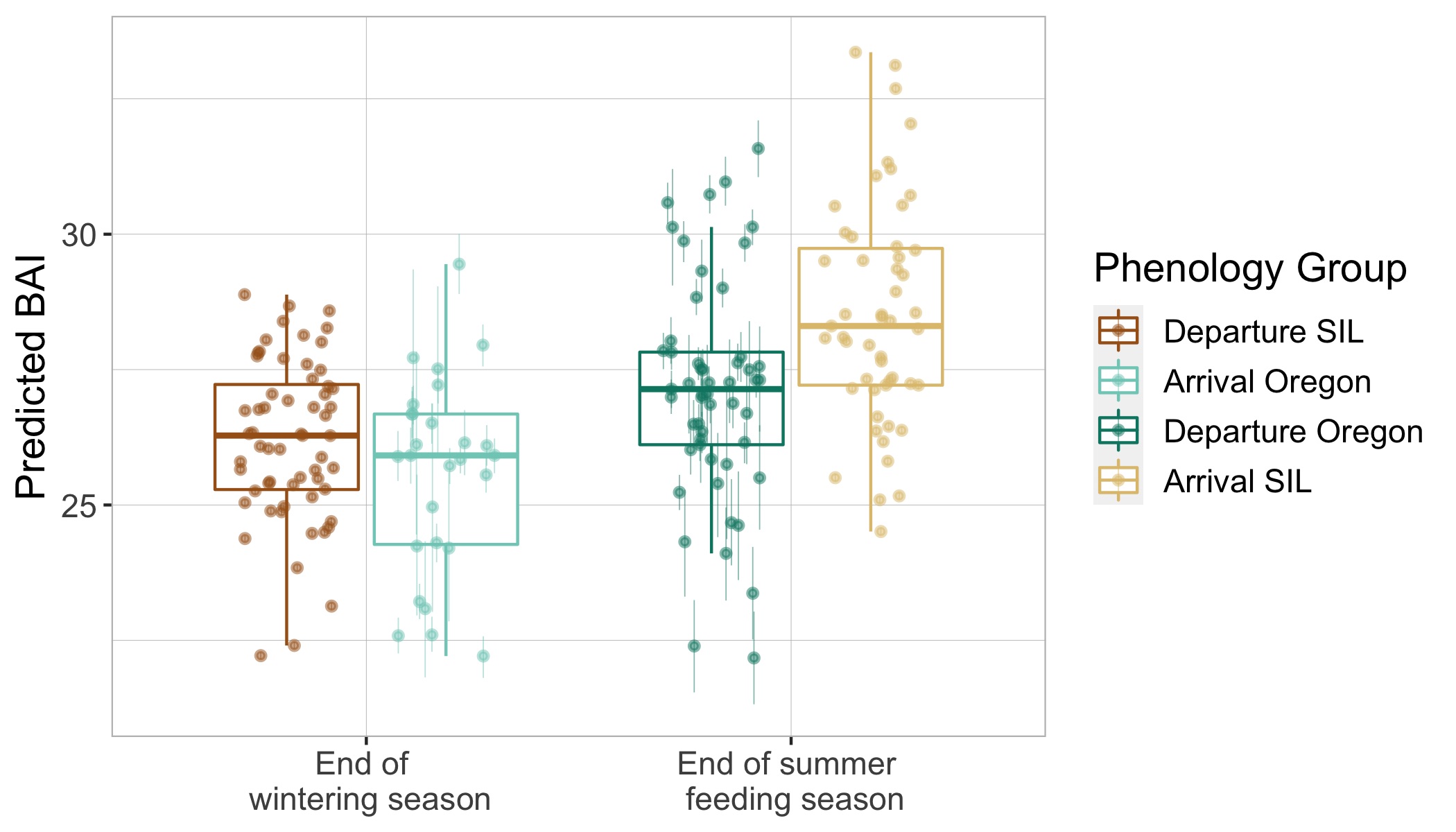
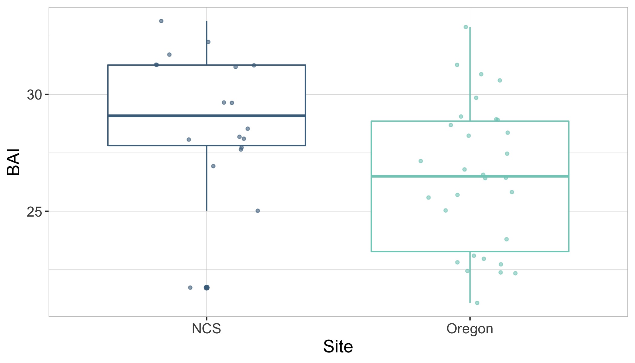
Surprisingly, the body condition of PCFG gray whales in Oregon was regularly and significantly lower than whales in San Ignacio Lagoon (Fig. 2). To further investigate this potential intrinsic difference in body condition between PCFG and ENP whales, we compared opportunistic photographs of gray whales feeding in the Northeastern Chukchi Sea (NCS) in the Arctic collected from airplane surveys. We found that the body condition of PCFG gray whales was significantly lower than whales in the NCS, further supporting our finding that PCFG whales overall have lower body condition than ENP whales that feed in the Arctic (Fig. 3).
Figure 2. Boxplots showing the distribution of Body Area Index (BAI) values for gray whales imaged by drones in San Ignacio Lagoon (SIL), Mexico and Oregon, USA. The data is grouped by phenology group: End of summer feeding season (departure Oregon vs. arrival SIL) and End of wintering season (arrival Oregon vs. departure SIL). The group median (horizontal line), interquartile range (IQR, box), maximum and minimum 1.5*IQR (vertical lines), and outliers (dots) are depicted in the boxplots. The overlaid points represent the mean of the posterior predictive distribution for BAI of an individual and the bars represents the uncertainty (upper and lower bounds of the 95% HPD interval). Note how PCFG whales at then end of the feeding season (dark green) typically have lower body condition (as BAI) compared to ENP whales at the end of the feeding season when they arrive to SIL after migration (light brown).Figure 3. Boxplots showing the distribution of Body Area Index (BAI) values of gray whales from opportunistic images collected from a plane in Northeaster Chukchi Sea (NCS) and from drones collected by the GEMM Lab in Oregon. The boxplots display the group median (horizontal line), interquartile range (IQR box), maximum and minimum 1.5*IQR (vertical lines), and outlies (dots). The overlaid points are the BAI values from each image. Note the significantly lower BAI of PCFG whales on Oregon feeding grounds compared to whales feeding in the Arctic region of the NCS.
This difference in body condition between PCFG and ENP gray whales raises some really interesting and prudent questions. Does the lower body condition of PCFG whales make them less resilient to changes in prey availability compared to ENP whales, and thus more vulnerable to climate change? If so, could this influence the reproductive capacity of PCFG whales? Or, are whales that recruit into the PCFG adapted to a smaller morphology, perhaps due to their specialized foraging tactics, which may be genetically inherited and enables them to survive with reduced energy stores?
These questions are on our minds here at the GEMM Lab as we prepare for our seventh consecutive field season using drones to collect data on PCFG gray whale body condition. As discussed in a previous blog by Dr. Alejandro Fernandez Ajo, we are combining our sightings history of individual whales, fecal hormone analyses, and photogrammetry-based body condition to better understand gray whales’ reproductive biology and help determine what the consequences are for these PCFG whales with lower body condition.
Did you enjoy this blog? Want to learn more about marine life, research, and conservation? Subscribe to our blog and get a weekly message when we post a new blog. Just add your name and email into the subscribe box below.
References
Bierlich, K. C., Hewitt, J., Bird, C. N., Schick, R. S., Friedlaender, A., Torres, L. G., … & Johnston, D. W. (2021). Comparing Uncertainty Associated With 1-, 2-, and 3D Aerial Photogrammetry-Based Body Condition Measurements of Baleen Whales. Frontiers in Marine Science, 1729.
Bierlich, K. C., Schick, R. S., Hewitt, J., Dale, J., Goldbogen, J. A., Friedlaender, A.S., et al. (2021b). Bayesian Approach for Predicting Photogrammetric Uncertainty in Morphometric Measurements Derived From Drones. Mar. Ecol. Prog. Ser. 673, 193–210. doi: 10.3354/meps13814
Burnett, J. D., Lemos, L., Barlow, D., Wing, M. G., Chandler, T., & Torres, L. G. (2018). Estimating morphometric attributes of baleen whales with photogrammetry from small UASs: A case study with blue and gray whales. Marine Mammal Science, 35(1), 108–139.
Christiansen, F., Rodrı́guez-González, F., Martı́nez-Aguilar, S., Urbán, J., Swartz, S., Warick, H., et al. (2021). Poor Body Condition Associated With an Unusual Mortality Event in Gray Whales. Mar. Ecol. Prog. Ser. 658, 237–252. doi:10.3354/meps13585
Hildebrand, L., Bernard, K. S., and Torres, L. G. (2021). Do Gray Whales Count Calories? Comparing Energetic Values of Gray Whale Prey Across Two Different Feeding Grounds in the Eastern North Pacific. Front. Mar. Sci. 8. doi: 10.3389/fmars.2021.683634
Stewart, J. D., and Weller, D. (2021). Abundance of Eastern North Pacific Gray Whales 2019/2020 (San Diego, CA: NOAA/NMFS)
Sumich, J. L. (1983). Swimming Velocities, Breathing Patterns, and Estimated Costs of Locomotion in Migrating Gray Whales, Eschrichtius Robustus. Can. J. Zoology. 61, 647–652. doi: 10.1139/z83-086
Torres, L.G., Bird, C., Rodrigues-Gonzáles, F., Christiansen F., Bejder, L., Lemos, L., Urbán Ramírez, J., Swartz, S., Willoughby, A., Hewitt., J., Bierlich, K.C. (2022). Range-wide comparison of gray whale body condition reveals contrasting sub-population health characteristics and vulnerability to environmental change. Frontiers in Marine Science. 9:867258. https://doi.org/10.3389/fmars.2022.867258
Allison Dawn, new GEMM Lab Master’s student, OSU Department of Fisheries, Wildlife and Conservation Sciences, Geospatial Ecology of Marine Megafauna Lab
While standing at the Stone Shelter at the Saint Perpetua Overlook in 2016, I took in the beauty of one of the many scenic gems along the Pacific Coast Highway. Despite being an East Coast native, I felt an unmistakable draw to Oregon. Everything I saw during that morning’s hike, from the misty fog that enshrouded evergreens and the ocean with mystery, to the giant banana slugs, felt at once foreign and a place I could call home. Out of all the places I visited along that Pacific Coast road trip, Oregon left the biggest impression on me.
Figure 1. View from the Stone Shelter at the Cape Perpetua Overlook, Yachats, OR. June 2016.
For my undergraduate thesis, which I recently defended in May 2021, I researched blue whale surface interval behavior. Surface interval events for oxygen replenishment and rest are a vital part of baleen whale feeding ecology, as it provides a recovery period before they perform their next foraging dive (Hazen et al., 2015; Roos et al., 2016). Despite spending so much time studying the importance of resting periods for mammals, that 2016 road trip was my last true extended resting period/vacation until, several years later in 2021, I took another road trip. This time it was across the country to move to the place that had enraptured me.
Now that I am settled in Corvallis, I have reflected on my journey to grad school and my recent road trip; both prepared me for a challenging and exciting new chapter as an incoming MSc student within the Marine Mammal Institute (MMI).
Part 1: Journey to Grad School
When I took that photo at the Cape Perpetua Overlook in 2016, I had just finished the first two semesters of my undergraduate degree at UNC Chapel Hill. As a first-generation, non-traditional student those were intense semesters as I made the transition from a working professional to full-time undergrad.
By the end of my freshman year I was debating exactly what to declare as my major, when one of my marine science TA’s, Colleen, (who is now Dr. Bove!), advised that I “collect experiences, not degrees.” I wrote this advice down in my day planner and have never forgotten it. Of course, obtaining a degree is important, but it is the experiences you have that help lead you in the right direction.
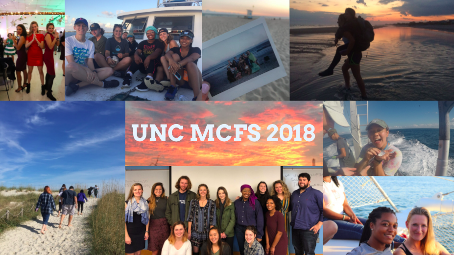
That advice was one of the many reasons I decided to participate in the Morehead City Field Site program, where UNC undergraduates spend a semester at the coast, living on the Duke Marine Lab’s campus in Beaufort, NC. During that semester, students take classes to fulfill a marine science minor while participating in hands-on research, including an honors thesis project. The experience of designing, carrying out, and defending my own project affirmed that graduate school in the marine sciences was right for me. As I move into my first graduate TA position this fall, I hope to pay forward that encouragement to other undergraduates who are making decisions about their own future path.
Figure 2. Final slide from my honors thesis defense. UNC undergraduates, and now fellow alumni, who participated in the Morehead City Field Site program in Fall 2018.
Part 2: Taking a Breather
Like the GEMM Lab’s other new master’s student Miranda, my road trip covered approximately 2,900 miles. I was solo for much of the drive, which meant there was no one to argue when I decided to binge listen to podcasts. My new favorite is How To Save A Planet, hosted by marine biologist Dr. Ayana Elizabeth Johnson and Alex Blumberg. At the end of each episode they provide a call to action & resources for listeners – I highly recommend this show to anyone interested in what you can do right now about climate change.
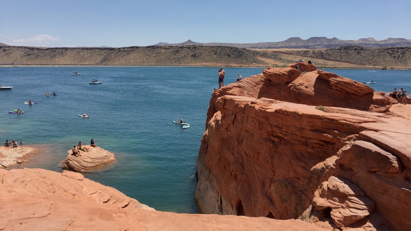
Along my trip I took a stop in Utah to visit my parents. I had never been to a desert basin before and engaged in many desert-related activities: visiting Zion National Park, hiking in 116-degree heat, and facing my fear of heights via cliff jumping.
Figure 3. Sandstone Rocks at Sand Hollow National Park, Hurricane, Utah. June 2021.
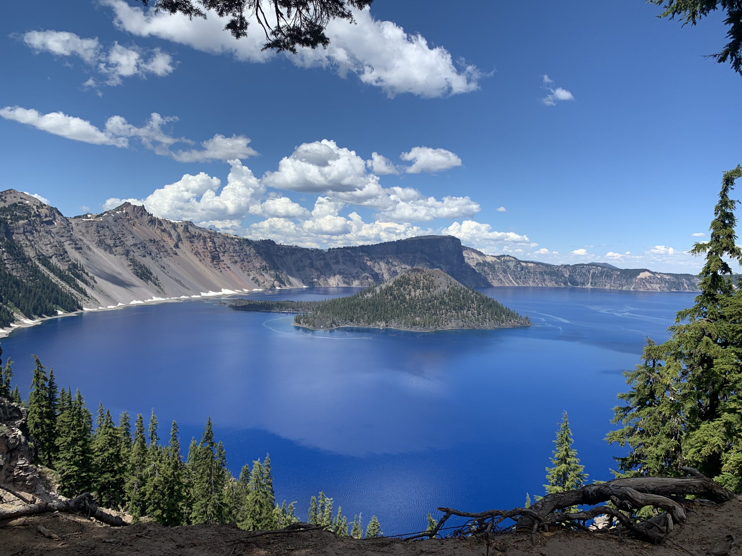
My parents wanted to help me settle into my new home, as parents do, so we drove the rest of the way to Oregon together. As this would be their first visit to the state, we strategically planned a trip to Crater Lake as our final scenic stop before heading into Corvallis.
Figure 4. Wizard Island in Crater Lake National Park, Klamath County, OR. June 2021.
This time off was filled with adventure, yet was restorative, and reminded me the importance of taking a break. I feel ready and refreshed for an intense summer of field work.
Part 3: Rested and Ready
Despite accumulating skills to do research in the field over the years, I have yet to do marine mammal field work (or even see a whale in person for that matter.) My mammal research experience included analyzing drone imagery, behind a computer, that had already been captured. As you can imagine, I am extremely excited to join the Port Orford team as part of the TOPAZ/JASPER projects this summer, collecting ecological data on gray whales and their prey. I will be learning the ropes from Lisa Hildebrand and soaking up as much information as possible as I will be taking over as lead for this project next year.
It will take some time before my master’s thesis is fully developed, but it will likely focus on assessing the environmental factors that influence gray whale zooplankton prey availability, and the subsequent impacts on whale movements and health. For five years, the Port Orford project has conducted GoPro drops at 12 sampling stations to collect data on zooplankton relative abundance.
Figures 5 & 6. GEMM GoPro drop stick assembly and footage demonstrating mysid data collection. July 2021.
Paired with this GoPro is a Time-Depth Recorder (TDR) that provides temperature and depth data. The 2021 addition to this GoPro system is a new dissolved oxygen (DO) sensor the GEMM Lab has just acquired. This new piece of equipment will add to the set of parameters we can analyze to describe what and how oceanographic factors drive prey variability and gray whale presence in our study site.My first task as a GEMM Lab student is to get to know this DO sensor, figure out how it works, set it up, test it, attach it to the GoPro device, and prepare it for data collection during the upcoming Port Orford project starting in 1 week!
Figure 7. The GEMM lab’s new RBR solo3 getting ready for Port Orford. July 2021.
Dissolved oxygen plays a vital role in the ocean; however, climate change and increased nutrient loading has caused the ocean to undergo deoxygenation. According to the IUCN’s 2019 Issues Brief, these factors have resulted in an oxygen decline of 2% since the middle of the 20th century, with most of this loss occurring within the first 1000 meters of the ocean. Two percent may not seem like much, but many species have a narrow oxygen threshold and, like pH changes in coral reef systems, even slight changes in DO can have an impact. Additionally, the first 1000 meters of the ocean contains the greatest amount of species richness and biodiversity.
Previous research done in a variety of systems (i.e., estuarine, marine, and freshwater lakes) shows that dissolved oxygen concentrations can have an impact on predator-prey interactions, where low dissolved oxygen results in decreased predation (Abrahams et al., 2007; Breitburg et al., 1997; Domenici et al., 2007; Kramer et al., 1987); and changes in DO also change prey vertical distributions (Decker et al., 2004). In Port Orford, we are interested in understanding the interplay of factors driving zooplankton community distribution and abundance while investigating the trophic interaction between gray whales and their prey.
I have spent some time with our new DO sensor and am looking forward to its first deployments in Port Orford! Stay tuned for updates from the field!
References
Abrahams, M. V., Mangel, M., & Hedges, K. (2007). Predator–prey interactions and changing environments: who benefits?. Philosophical Transactions of the Royal Society B: Biological Sciences, 362(1487), 2095-2104.
Breitburg, D. L., Loher, T., Pacey, C. A., & Gerstein, A. (1997). Varying effects of low dissolved oxygen on trophic interactions in an estuarine food web. Ecological Monographs, 67(4), 489-507.
Decker, M. B., Breitburg, D. L., & Purcell, J. E. (2004). Effects of low dissolved oxygen on zooplankton predation by the ctenophore Mnemiopsis leidyi. Marine Ecology Progress Series, 280, 163-172.
Domenici, P., Claireaux, G., & McKenzie, D. J. (2007). Environmental constraints upon locomotion and predator–prey interactions in aquatic organisms: an introduction.
Hazen, E. L., Friedlaender, A. S., & Goldbogen, J. A. (2015). Blue whales (Balaenoptera musculus) optimize foraging efficiency by balancing oxygen use and energy gain as a function of prey density. Science Advances, 1(9), e1500469.
Kramer, D. L. (1987). Dissolved oxygen and fish behavior. Environmental biology of fishes, 18(2), 81-92.
Roos, M. M., Wu, G. M., & Miller, P. J. (2016). The significance of respiration timing in the energetics estimates of free-ranging killer whales (Orcinus orca). Journal of Experimental Biology, 219(13), 2066-2077.
Clara Bird, PhD Student, OSU Department of Fisheries and Wildlife, Geospatial Ecology of Marine Megafauna Lab
In order to understand a species’ distribution, spatial ecologists assess which habitat characteristics are most often associated with a species’ presence. Incorporating behavior data can improve this analysis by revealing the functional use of each habitat type, which can help scientists and managers assign relative value to different habitat types. For example, habitat used for foraging is often more important than habitat that a species just travels through. Further complexity is added when we consider that some species, such as gray whales, employ a variety of foraging tactics on a variety of prey types that are associated with different habitats. If individual foraging tactic specialization is present, different foraging habitats could be valuable to specific subgroups that use each tactic. Consequently, for a population that uses a variety of foraging tactics, it’s important to study the associations between tactics and habitat characteristics.
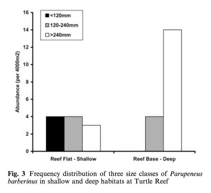
Lukoschek and McCormick’s (2001) study investigating the spatial distribution of a benthic fish species’ foraging behavior is a great example of combining data on behavior, habitat, and morphology. They collected data on the diet composition of individual fish categorized into different size classes (small, medium, and large) and what foraging tactics were used in which reef zones and habitat types. The foraging tactics ranged from feeding in the water column to digging (at a range of depths) in the benthic substrate. The results showed that an interesting combination of fish behavior and morphology explained the observed diet composition and spatial distribution patterns. Small fish foraged in shallower water, on smaller prey, and primarily employed the water column and shallow digging tactics. In contrast, large fish foraged in deep water, on larger prey, and primarily fed by digging deeper into the seafloor (Figure 1). This pattern is explained by both morphology and behavior. Morphologically, the size of the feeding apparatus (mouth gape size) affects the size of the prey that a fish can feed on. The gape of the small fish is not large enough to eat the larger prey that large fish are able to consume. Behaviorally, predation risk also affects habitat selection and tactic use. Small fish are at higher risk of being predated on, so they remain in shallow areas where they are more protected from predators and they don’t dig as deep to forage because they need to be able to keep an eye out for predators. Interestingly, while they found a relationship between the morphology of the fish and habitat use, they did not find an association between specific feeding tactics and habitat types.
Figure 1. Figure from Lukoschek and McCormick (2001) showing that small fish (black bar) were found in shallow habitat while large fish (white bar) were found in deep habitat.
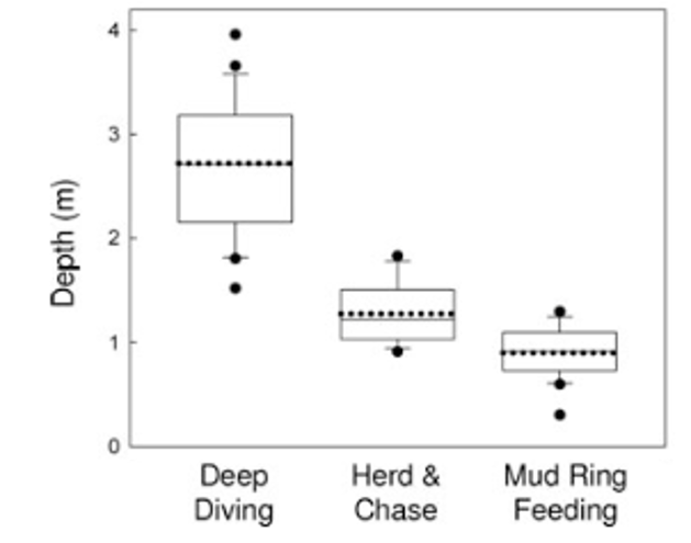
Conversely, Torres and Read (2009) did find associations between theforaging tactics of bottlenose dolphins in Florida Bay, FL and habitat type. Dolphins in this bay employ three foraging tactics: herd and chase, mud ring feeding, and deep diving. Observations of the foraging tactics were linked to habitat characteristics and individual dolphins. The study found that these tactics are spatially structured by depth (Figure 2), with deep diving occurring in deep water whereas mud ring feeding occurrs in shallower water. They also found evidence of individual specialization! Individuals that were observed deep diving were not observed mud ring feeding and vice-versa. Furthermore, they found that individuals were found in the habitat type associated with their preferred tactic regardless of whether they were foraging or not. This result indicates that individual dolphins in this bay have a foraging tactic they prefer and tend to stay in the corresponding habitat type. These findings are really intriguing and raise interesting questions regarding how these tactics and specializations are developed or learned. These are questions that I am also interested in asking as part of my thesis.
Figure 2. Figure from Torres and Read (2009) showing that deep diving is associated with deeper habitat while mud ring feeding is associated with shallow habitat.
Both of these studies are cool examples that, combined, exemplify questions I am interested in examining using our study population of Pacific Coast Feeding Group (PCFG) gray whales. Like both studies, I am interested in assessing how specific foraging tactics are associated with habitat types. Our hypothesis is that different prey types live in different habitat types, so each tactic corresponds to the best way to feed on that prey type in that habitat. While predation risk doesn’t have as much of an effect on foraging gray whales as it does on small benthic fish, I do wonder how disturbance from boats could similarly affect tactic preference and spatial distribution. I am also curious to see if depth has an effect on tactic choice by using the morphology data from our drone-based photogrammetry. Given that these whales forage in water that is sometimes as deep as they are long, it stands to reason that maneuverability would affect tactic use. As described in a previous blog, I’m also looking for evidence of individual specialization. It will be fascinating to see how foraging preference relates to space use, habitat preference, and morphology.
These studies demonstrate the complexity involved in studying a population’s relationship to its habitat. Such research involves considering the morphology and physiology of the animals, their social, individual, foraging, and predator-prey behaviors, and the relationship between their prey and the habitat. It’s a bit daunting but mostly really exciting because better understanding each puzzle piece improves our ability to estimate how these animals will react to changing environmental conditions.
While I don’t have any answers to these questions yet, I will be working with a National Science Foundation Research Experience for Undergraduates intern this summer to develop a habitat map of our study area that will be used in this analysis and potentially answer some preliminary questions about PCFG gray whale habitat use patterns. So, stay tuned to hear more about our work this summer!
References
Lukoschek, V., & McCormick, M. (2001). Ontogeny of diet changes in a tropical benthic carnivorous fish, Parupeneus barberinus (Mullidae): Relationship between foraging behaviour, habitat use, jaw size, and prey selection. Marine Biology, 138(6), 1099–1113. https://doi.org/10.1007/s002270000530
Torres, L. G., & Read, A. J. (2009). Where to catch a fish? The influence of foraging tactics on the ecology of bottlenose dolphins ( Tursiops truncatus ) in Florida Bay, Florida. Marine Mammal Science, 25(4), 797–815. https://doi.org/10.1111/j.1748-7692.2009.00297.x
By: Alexa Kownacki, Ph.D. Student, OSU Department of Fisheries and Wildlife, Geospatial Ecology of Marine Megafauna Lab
Humans are fascinated by food. We want to know its source, its nutrient content, when it was harvested and by whom, and so much more. Since childhood, I was the nagging child who interrogated wait staff about the seafood menu because I cared about the sustainability aspect as well as consuming ethically-sourced seafood. Decades later I still do the same: ask a myriad of questions from restaurants and stores in order to eat as sustainably as possible. But in addition to asking these questions about my food, I also question what my study species eats and why. My study populations, common bottlenose dolphins, are described as top opportunistic predators (Norris and Prescott 1961, Shane et al. 1986, Barros and Odell 1990). In my study area off of California, this species exists in two ecotypes. The coastal ecotype off of California, USA are generalist predators, feeding on many different species of fish using different foraging techniques (Ballance 1992, Shane 1990). The offshore ecotype, on the other hand, is less well-studied, but is frequently observed in association with sperm whales, although the reason is still unknown (Díaz-Gamboa et al. 2018). Stable isotope analysis from skin samples from the two ecotypes indicates that the ecotypes exhibit different foraging strategies based on different isotopic carbon and nitrogen levels (Díaz-Gamboa et al. 2018).
Growing up, I kept the Monterey Bay Aquarium’s Seafood Watch Guide with me to choose the most sustainably-sourced seafood at restaurants. Today there is an easy-to-use application for mobile phones that replaced the paper guide. (Image Source: https://www.seafoodwatch.org/)
Preliminary and historical data on common bottlenose dolphins (Tursiops truncatus) suggest that the coastal ecotype spend more time near estuary mouths than offshore dolphins (Ballance 1992, Kownacki et al. unpublished data). Estuaries contain large concentrations of nutrients from runoff, which support zooplankton and fishes. It is for this reason that these estuaries are thought to be hotspots for bottlenose dolphin foraging. Some scientists hypothesize that these dolphins are estuarine-based prey specialists (Barros and Odell 1990), or that the dolphins simply aggregate in estuaries due to higher prey abundance (Ballance 1992).
Coastal bottlenose dolphins traveling near an estuary mouth in San Diego, CA. (Photographed under NOAA NMFS Permit # 19091).
In an effort to understand diet compositions of bottlenose dolphins, during coastal surveys seabirds were recorded in association with feeding groups of dolphins. Therefore, it is reasonable to believe that dolphins were feeding on the same fishes as Brown pelicans, blue-footed and brown boobies, double-crested cormorants, and magnificent frigatebirds, seeing as they were the most common species associated with bottlenose dolphin feeding groups (Ballance 1992). A shore-based study by Hanson and Defran (1993) found that coastal dolphins fed more often in the early morning and late afternoon, as well as during periods of high tide current. These patterns may have to do with the temporal and spatial distribution of prey fish species. From the few diet studies conducted on these bottlenose dolphins in this area, 75% of the prey were species from the families Ebiotocidae (surf perches) and Sciaendae (croakers) (Norris and Prescott 1961, Walker 1981). These studies, in addition to optimal foraging models, suggest this coastal ecotype may not be as much of a generalist as originally suggested (Defran et al. 1999).
A redtail surfperch caught by a fisherman from a beach in San Diego, CA. These fish are thought to be common prey of coastal bottlenose dolphins. (Image Source: FishwithJD)
Diet studies on the offshore ecotype of bottlenose dolphins worldwide show a preference for cephalopods, similar to other toothed cetaceans who occupy similar regions, such as Risso’s dolphin, sperm whales, and pilot whales (Clarke 1986, Cockcroft and Ross 1990, Gonzalez et al. 1994, Barros et al. 2000, Walker et al. 1999). Because these animals seldom strand on accessible beaches, stomach contents analyses are limited to few studies and isotope analysis is more widely available from biopsies. We know these dolphins are sighted in deeper waters than the habitat of coastal dolphins where there are fewer nutrient plumes, so it is reasonable to hypothesize that the offshore ecotype consumes different species and may be more specialized than the coastal ecotype.
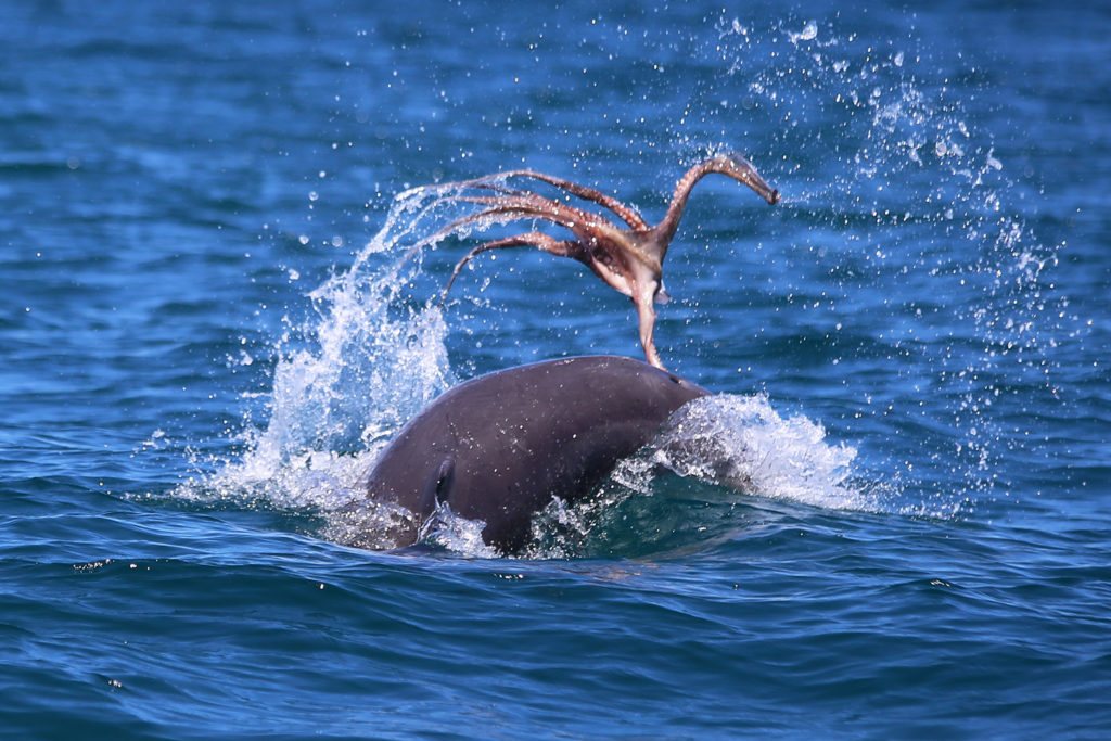
An bottlenose dolphin forages on an octopus. (Image source: Mandurah Cruises)
For a species that is so often observed from shore and boats, and is known for its charisma, it may be surprising that the diets of both the coastal and offshore bottlenose dolphins are still largely unknown. Such is the challenge of studying animals that live and feed underwater. I wish I could simply ask a dolphin, much like I would ask staff at restaurants: what is on the menu today? But, unfortunately, that is not possible. Instead, we must make educated hypotheses about the diets of both ecotypes based on necropsies and stable isotope studies, and behavioral and spatial surveys. And, I will continue to look to new technologies and creative thinking to provide the answers we are seeking.
Literature cited:
Ballance, L. T. (1992). Habitat use patterns and ranges of the bottlenose dolphin in the Gulf of California, Mexico. Marine Mammal Science, 8(3), 262-274.
Barros, N.B., and D. K. Odell. (1990). Food habits of bottlenose dolphins in the southeastern United States. Pages 309-328 in S. Leatherwood and R. R. Reeves, eds. The bottlenose dolphin. Academic Press, San Diego, CA.
Barros, N., E. Parsons and T. Jefferson. (2000). Prey of bottlenose dolphins from the South China Sea. Aquatic Mammals 26:2–6.
Clarke, M. 1986. Cephalopods in the diet of odontocetes. Pages 281–321 in M. Bryden and R. Harrison, eds. Research on dolphins. Clarendon Press, Oxford, NY.
Cockcroft, V., and G. Ross. (1990). Food and feeding of the Indian Ocean bottlenose dolphin off southern Natal, South Africa. Pages 295–308 in S. Leatherwood and R. R. Reeves, eds. The bottlenose dolphin. Academic Press, San Diego, CA.
Defran, R. H., Weller, D. W., Kelly, D. L., & Espinosa, M. A. (1999). Range characteristics of Pacific coast bottlenose dolphins (Tursiops truncatus) in the Southern California Bight. Marine Mammal Science, 15(2), 381-393.
Díaz‐Gamboa, R. E., Gendron, D., & Busquets‐Vass, G. (2018). Isotopic niche width differentiation between common bottlenose dolphin ecotypes and sperm whales in the Gulf of California. Marine Mammal Science, 34(2), 440-457.
Gonzalez, A., A. Lopez, A. Guerra and A. Barreiro. (1994). Diets of marine mammals stranded on the northwestern Spanish Atlantic coast with special reference to Cephalopoda. Fisheries Research 21:179–191.
Hanson, M. T., and Defran, R. H. (1993). The behavior and feeding ecology of the Pacific coast bottlenose dolphin, Tursiops truncatus. Aquatic Mammals, 19, 127-127.
Norris, K. S., and J. H. Prescott. (1961). Observations on Pacific cetaceans of Californian and Mexican waters. University of California Publications of Zoology 63:29, 1-402.
Shane, S. H. (1990). Comparison of bottlenose dolphin behavior in Texas and Florida, with a critique of methods for studying dolphin behavior. Pages 541-558 in S. Leatherwood and R. R. Reeves, eds. The bottlenose dolphin. Academic Press, San Diego, CA.
Shane, S., R. Wells and B. Wursig. (1986). Ecology, behavior and social organization of bottlenose dolphin: A review. Marine Mammal Science 2:34–63.
Walker, W.A. (1981). Geographical variation in morphology and biology of the bottlenose dolphins (Tursiops) in the eastern North Pacific. NMFS/SWFC Administrative Report. No, LJ-91-03C.
Walker, J., C. Potter and S. Macko. (1999). The diets of modern and historic bottlenose dolphin populations reflected through stable isotopes. Marine Mammal Science 15:335–350.
By Hunter Warick, Research Technician, Geospatial Ecology of Marine Megafauna Lab, Marine Mammal Institute
When monitoring the health of a capital breeding species, such as whales that store energy to support reproduction costs, it is important to understand what processes and factors drive the status of their body condition. Information gained will allow for better insight into their cost of reproduction and overall life history strategies.
For the past four years the GEMM Lab has utilized the perspective that Unoccupied Aerial Systems (UAS; or ‘drones’) provide for observations of marine mammals. This aerial perspective has documented gray whale behavior such as jaw snapping, drooling mud, and headstands, all of which shows or suggest foraging (Torres et al. 2018). However, UAS is limited to a bird’s eye view, allowing us to see WHAT whales are doing, but limited information about the reasons WHY. To overcome this hurdle, Leigh Torres and team have equipped their marine mammal research utility belts with the use of GoPro cameras. They developed a technique known as the “GoPro drop” where a GoPro camera mounted to a weighted pole is lowered off the side of the research vessel in waters < 20 m deep via a line to record video data. This technique allows the team to obtain fine-scale habitat and prey variation information, like what the whale experiences. Along with the context provided by the UAS, this dual camera perspective allows for deeper insight into gray whale foraging strategies and efficiency. Torres’s GoPro data analysis protocol examines kelp density, kelp health, benthic substrate, rock fish density, and mysid density. These characteristics are graded along a scale (Figure 1), allowing for relative comparisons of habitat and prey availability between where whales spend time and forage. These GoPro drops will also help create a fine-scale benthic habitat map of the Newport field area. So, why are these data on gray whale habitat and prey important to understand?
Figure 1. The top row shows varying degrees of mysid density (low to high, left to right). Middle row illustrates different types of substrate you might encounter (reef, sandy, boulders; left to right). Bottom row shows the different levels of kelp health (poor, medium, good).
The foraging grounds are the first step in the life history domino chain reaction for many rorqual whales; if this step doesn’t go off cleanly then everything else fails to fall into place. Gray whales partake on a 15,000-20,000 km (round trip) migration, which is the longest of any known mammal (Swartz 1986). During this migration, whales spend around three months fasting in their breeding grounds (Highsmith & Coyle 1992), living only off the energy stores that they accumulated in their feeding grounds (Næss et al. 1998). These extreme conditions of existence for gray whales drive the need to be a successful forager and is why it is so crucial for them to forage in high prey density areas (Newell, C. 2009).
Mysids are a critical part of the gray whale diet in Oregon waters (Newell, C. 2009; Sullivan, F. 2017) and mysids have strong predator-prey relationships with both top-down and bottom-up control (Dunham & Duffus 2001; Newell & Cowles 2006). This unique tie illustrates the great dependency that gray whales have on mysids, further showing the benefit to looking at the density of mysids where gray whales are seen foraging. The quality of mysids may also be as important as quantity; with higher water temperatures resulting in lower lipid content in mysids (Mauchline 1980), suggesting density might not be the only factor for determining efficient whale foraging. The overall goal of gray whales on their foraging grounds is to get as fat as possible in order to reproduce as often as possible. But, this isn’t always as easy as it sounds. Gray whales typically have a two-year breeding interval but can be anywhere from 1-4 years (Blokhin 1984). The longer time it takes to build up adequate energy stores to support reproduction costs, the longer it will take to breed successfully. Building back up these energy stores can prove to be difficult, especially for lactating females (Figure 2).
Figure 2. Comparison of body condition between a lactating female gray whale on the feeding grounds in Newport, Oregon, 2020 (GEMM Lab, OSU; NOAA/NMFS permit # 21678) and a pregnant female gray whale on the breeding grounds in San Ignacio Lagoon, 2019 (provided by Laguna San Ignacio Ecosystem Program). Photographer Hunter Warick. Note the very different body shapes: thin lactating female relative to the rotund pregnant female.
Being able to track the health and behavior of gray whales on an individual level, including comparisons between variation in body condition, foraging behavior, and fine scale information on benthic communities gained through the use of GoPros, can provide a better understanding of the driving factors and impacts on their health and population trends (Figure 3).
Figure 3. A compilation of video clips captured by the GEMM Lab during their research on gray whale ecology and physiology off Newport, Oregon using Unoccupied Aerial Systems (UAS, or “drones”) and GoPro cameras. UAS are used to observe gray whale behavior and conduct photogrammetry assessment of body condition. GoPro camera drops assess the benthic habitat and prey density across the study region, with a couple chance encounters of whales. Research is conducted under NOAA/NMFS permit # 21678.
In the GEMM Lab, our research focuses largely on the ecology of marine top predators. Inherent in our work are often assumptions that our study species—wide-ranging predators including whales, dolphins, otters, or seabirds—will distribute themselves relative to their prey. In order to make a living in the highly patchy and dynamic marine environment, predators must find ways to predictably locate and exploit prey resources.
But what about the prey? How do the prey structure themselves relative to their predators? This question is explored in depth in a paper titled “The Landscape of Fear: Ecological Implications of Being Afraid” (Laundre et al. 2010), which we discussed in our most recent lab meeting. When wolves were re-introduced in Yellowstone, the elk increased their vigilance and altered their grazing patterns. As a result, the plant community was altered to reflect this “landscape of fear” that the elk move through, where their distribution not only reflected opportunities for the elk to eat but also the risk of being eaten.
Translating the landscape of fear concept to the marine environment is tricky, but a fascinating exercise in ecological theory. We grappled with drawing parallels between the example system of wolves, elk, and vegetation and baleen whales, zooplankton, and phytoplankton. Relative to grazing mammals like elk, the cognitive abilities of zooplankton like krill, copepods, and mysid might pale in comparison. How could we possibly measure “fear” or “vigilance” in zooplankton? The swarming behavior of mysid and krill into dense patches is a defense mechanism—the strategy they have evolved to lessen the likelihood that any one of them will be eaten by a predator. I would posit that the diel vertical migration (DVM) of zooplankton is a manifestation of fear, at least on some level. DVM occurs over the course of each day, with plankton in pelagic ecosystems migrating vertically in the water column to avoid predators by hiding at depth during the daylight hours, and then swimming upward to feed on phytoplankton under the cover of darkness. I won’t speculate any further on the intelligence of zooplankton, but the need to survive predation has driven them to evolve this effective evolutionary strategy of hiding in the ocean’s twilight zone, swimming upward to feed only after dark so that they’re less likely to linger in spaces occupied by predators.
A swarm of mysid along the Oregon Coast. How does fear of predation by gray whales or rockfish drive the distribution of zooplankton in this shallow, nearshore system? Photo by Dawn Barlow.
A rock covered in purple urchin on the Oregon Coast. In the absence of their major predators (sea otters and sea stars), are urchins able to thrive in an environment with less fear of predation? Photo by Dawn Barlow.
A blue whale lunges on a dense aggregation of krill in New Zealand. In this image, you can actually see the krill “fleeing”, jumping out of the water in an attempt to escape the whale’s mouth. Drone piloted by Todd Chandler.
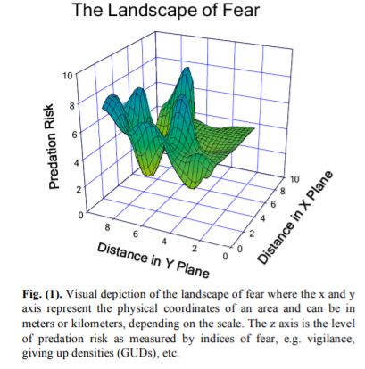
Laundre et al. (2010) present a visual representation of the landscape of fear (Fig. 1, reproduced below), where as an animal moves through space (represented as distance in meters or kilometers, for example), they also move through varying levels of predation risk. Environmental gradients (temperature, for example) tend to be much more stable across space in terrestrial ecosystems such as in the Yellowstone example from the paper. I wonder whether the same concept and visual depiction of a landscape of fear could be translated as risk across various environmental gradients, rather than geographic distances? In this proposed illustration, a landscape of fear would vary based on gradients of environmental conditions rather than geographic space. Such a shift in spatial reference —from geographic to environmental space—might make the model more applicable in the dynamic ocean ecosystems that we study.
What about cases when the predators we study become prey? One example we discussed was gray whales migrating from breeding lagoons in Mexico to feeding grounds in the Bering Sea. Mother-calf pairs hug the coastline tightly, by no means taking the most direct route between locations and adding considerable travel distance to their migration. The leading hypothesis is that mother gray whales take the coastal route to minimize the risk that their calves will fall prey to killer whale attacks. Are there other cases where the predators we study operate in a seascape of fear that we do not yet understand? Likely so, and the predators’ own seascape of fear may account for cases when we cannot explain predator distribution simply by their prey and their environment. To take this a step further, it might be beneficial not only to think of predation risk as only the potential to be eaten, but expand our definition to include human disturbance. While humans may not directly prey on marine predators, the disturbance from human activity in the ocean likely creates a layer of fear which animals must navigate, even in the absence of actual predation.
Our lively lab meeting discussion prompted me to look into
how the landscape of fear model has been applied to the highly dynamic and
intricate marine environment. In a study examining predator-prey dynamics of
three species of marine mammals—bottlenose dolphins, harbor seals, and
dugongs—Wirsing et al. (2007) found that in all three cases, the study species
spent less time in more desirable prey patches or decreased riskier behavior in
the presence of predators. Most studies in marine ecology are observational, as
we rarely have the opportunity to manipulate our study system for experimental
design and hypothesis testing. However, a study of coral reefs in the Florida
Keys conducted by Catano et al. (2015) used fabricated predators—decoys of
black grouper, a predatory fish—to investigate the influence of fear of
predation on the reef system. What they found was that herbivorous fish
consumed significantly less and fed at a much faster rate in the presence of this
decoy predator. The grouper, even in decoy form, created a “reefscape of fear”,
altering patterns in herbivory with potential ramifications for the entire ecosystem.
My takeaway from our discussion and my musings in this
week’s blog post is that predator and prey distribution and behavior is highly
interconnected. While predators distribute themselves to maximize their ability
to find a meal, their prey respond accordingly by balancing finding a meal of
their own with minimizing the risk that they will be eaten. Ecology is the
study of an ecosystem, which means the questions we ask are complicated and
hierarchical, and must be considered from multiple angles, accounting for
biological, environmental, and behavioral elements to name a few. These
challenges of studying ecosystems are simultaneously what make ecology
fascinating, and exciting.
References:
Laundré, J. W., Hernández, L., & Ripple, W. J. (2010).
The landscape of fear: ecological implications of being afraid. Open
Ecology Journal, 3, 1-7.
Catano, L. B., Rojas, M. C., Malossi, R. J., Peters, J. R.,
Heithaus, M. R., Fourqurean, J. W., & Burkepile, D. E. (2016). Reefscapes
of fear: predation risk and reef hetero‐geneity interact to shape herbivore
foraging behaviour. Journal of Animal Ecology, 85(1),
146-156.
Wirsing, A. J., Heithaus, M. R., Frid, A., & Dill, L. M.
(2008). Seascapes of fear: evaluating sublethal predator effects experienced
and generated by marine mammals. Marine Mammal Science, 24(1),
1-15.
By: Alexa Kownacki, Ph.D. Student, OSU Department of Fisheries and Wildlife, Geospatial Ecology of Marine Megafauna Lab
Data analysis is often about parsing down data into manageable subsets. My project, which spans 34 years and six study sites along the California coast, requires significant data wrangling before full analysis. As part of a data analysis trial, I first refined my dataset to only the San Diego survey location. I chose this dataset for its standardization and large sample size; the bulk of my sightings, over 4,000 of the 6,136, are from the San Diego survey site where the transect methods were highly standardized. In the next step, I selected explanatory variable datasets that covered the sighting data at similar spatial and temporal resolutions. This small endeavor in analyzing my data was the first big leap into understanding what questions are feasible in terms of variable selection and analysis methods. I developed four major hypotheses for this San Diego site.
The study species: common bottlenose dolphin (Tursiops truncatus) seen along the California coastline in 2015. Image source: Alexa Kownacki.
Hypotheses:
H1: I predict that bottlenose dolphin sightings along the San Diego transect throughout the years 1981-2015 exhibit clustered distribution patterns as a result of the patchy distributions of both the species’ preferred habitats, as well as the social nature of bottlenose dolphins.
H2: I predict there would be higher densities of bottlenose dolphin at higher latitudes spanning 1981-2015 due to prey distributions shifting northward and less human activities in the northerly sections of the transect.
H3: I predict that during warm (positive) El Niño Southern Oscillation (ENSO) months, the dolphin sightings in San Diego would be distributed more northerly, predominantly with prey aggregations historically shifting northward into cooler waters, due to (secondarily) increasing sea surface temperatures.
H4: I predict that along the San Diego coastline, bottlenose dolphin sightings are clustered within two kilometers of the six major lagoons, with no specific preference for any lagoon, because the murky, nutrient-rich waters in the estuarine environments are ideal for prey protection and known for their higher densities of schooling fishes.
Data Description:
The common bottlenose dolphin (Tursiops truncatus) sighting data spans 1981-2015 with a few gap years. Sightings cover all months, but not in all years sampled. The same transect in San Diego was surveyed in a small, rigid-hulled inflatable boat with approximately a two-kilometer observation area (one kilometer surveyed 90 degrees to starboard and port of the bow).
I wanted to see if there were changes in dolphin distribution by latitude and, if so, whether those changes had a relationship to ENSO cycles and/or distances to lagoons. For ENSO data, I used the NOAA database that provides positive, neutral, and negative indices (1, 0, and -1, respectively) by each month of each year. I matched these ENSO data to my month-date information of dolphin sighting data. Distance from each lagoon was calculated for each sighting.
Figure 1. Map representing the San Diego transect, represented with a light blue line inside of a one-kilometer buffered “sighting zone” in pale yellow. The dark pink shapes are dolphin sightings from 1981-2015, although some are stacked on each other and cannot be differentiated. The lagoons, ranging in size, are color-coded. The transect line runs from the breakwaters of Mission Bay, CA to Oceanside Harbor, CA.
Results:
H1:True, dolphins are clustered and do not have a uniform distribution across this area. Spatial analysis indicated a less than a 1% likelihood that this clustered pattern could be the result of random chance (Fig. 1, z-score = -127.16, p-value < 0.0001). It is well-known that schooling fishes have a patchy distribution, which could influence the clustered distribution of their dolphin predators. In addition, bottlenose dolphins are highly social and although pods change in composition of individuals, the dolphins do usually transit, feed, and socialize in small groups.
Figure 2. Summary from the Average Nearest Neighbor calculation in ArcMap 10.6 displaying that bottlenose dolphin sightings in San Diego are highly clustered. When the z-score, which corresponds to different colors on the graphic above, is strongly negative (< -2.58), in this case dark blue, it indicates clustering. Because the p-value is very small, in this case, much less than 0.01, these results of clustering are strongly significant.
H2:False, dolphins do not occur at higher densities in the higher latitudes of the San Diego study site. The sightings are more clumped towards the lower latitudes overall (p < 2e-16), possibly due to habitat preference. The sightings are closer to beaches with higher human densities and human-related activities near Mission Bay, CA. It should be noted, that just north of the San Diego transect is the Camp Pendleton Marine Base, which conducts frequent military exercises and could deter animals.
Figure 3. Histogram comparing the latitudes with the frequency of dolphin sightings in San Diego, CA. The x-axis represents the latitudinal difference from the most northern part of the transect to each dolphin sighting. Therefore, a small difference would translate to a sighting being in the northern transect areas whereas large differences would translate to sightings being more southerly. This could be read from left to right as most northern to most southern. The y-axis represents the frequency of which those differences are seen, that is, the number of sightings with that amount of latitudinal difference, or essentially location on the transect line. Therefore, you can see there is a peak in the number of sightings towards the southern part of the transect line.
H3: False, during warm (positive) El Niño Southern Oscillation (ENSO) months, the dolphin sightings in San Diego were more southerly. In colder (negative) ENSO months, the dolphins were more northerly. The differences between sighting latitude and ENSO index was significant (p<0.005). Post-hoc analysis indicates that the north-south distribution of dolphin sightings was different during each ENSO state.
Figure 4. Boxplot visualizing distributions of dolphin sightings latitudinal differences and ENSO index, with -1,0, and 1 representing cold, neutral, and warm years, respectively.
H4:True, dolphins are clustered around particular lagoons. Figure 5 illustrates how dolphin sightings nearest to Lagoon 6 (the San Dieguito Lagoon) are always within 0.03 decimal degrees. Because of how these data are formatted, decimal degrees is the easiest way to measure change in distance (in this case, the difference in latitude). In comparison, dolphins at Lagoon 5 (Los Penasquitos Lagoon) are distributed across distances, with the most sightings further from the lagoon.
Figure 5. Bar plot displaying the different distances from dolphin sighting location to the nearest lagoon in San Diego in decimal degrees. Note: Lagoon 4 is south of the study site and therefore was never the nearest lagoon.
I found a significant difference between distance to nearest lagoon in different ENSO index categories (p < 2.55e-9): there is a significant difference in distance to nearest lagoon between neutral and negative values and positive and neutral years. Therefore, I hypothesize that in neutral ENSO months compared to positive and negative ENSO months, prey distributions are changing. This is one possible hypothesis for the significant difference in lagoon preference based on the monthly ENSO index. Using a violin plot (Fig. 6), it appears that Lagoon 5, Los Penasquitos Lagoon, has the widest variation of sighting distances in all ENSO index conditions. In neutral years, Lagoon 0, the Buena Vista Lagoon has multiple sightings, when in positive and negative years it had either no sightings or a single sighting. The Buena Vista Lagoon is the most northerly lagoon, which may indicate that in neutral ENSO months, dolphin pods are more northerly in their distribution.
Figure 6. Violin plot illustrating the distance from lagoons of dolphin sightings under different ENSO conditions. There are three major groups based on ENSO index: “-1” representing cold years, “0” representing neutral years, and “1” representing warm years. On the x-axis are lagoon IDs and on the y-axis is the distance to the nearest lagoon in decimal degrees. The wider the shapes, the more sightings, therefore Lagoon 6 has many sightings within a very small distance compared to Lagoon 5 where sightings are widely dispersed at greater distances.
Bottlenose dolphins foraging in a small group along the California coast in 2015. Image source: Alexa Kownacki.
Takeaways to science and management:
Bottlenose dolphins have a clustered distribution which seems to be related to ENSO monthly indices, and likely, their social structures. From these data, neutral ENSO months appear to have something different happening compared to positive and negative months, that is impacting the sighting distributions of bottlenose dolphins off the San Diego coastline. More research needs to be conducted to determine what is different about neutral months and how this may impact this dolphin population. On a finer scale, the six lagoons in San Diego appear to have a spatial relationship with dolphin sightings. These lagoons may provide critical habitat for bottlenose dolphins and/or for their preferred prey either by protecting the animals or by providing nutrients. Different lagoons may have different spans of impact, that is, some lagoons may have wider outflows that create larger nutrient plumes.
Other than the Marine Mammal Protection Act and small protected zones, there are no safeguards in place for these dolphins, whose population hovers around 500 individuals. Therefore, specific coastal areas surrounding lagoons that are more vulnerable to habitat loss, habitat degradation, and/or are more frequented by dolphins, may want greater protection added at a local, state, or federal level. For example, the Batiquitos and San Dieguito Lagoons already contain some Marine Conservation Areas with No-Take Zones within their reach. The city of San Diego and the state of California need better ways to assess the coastlines in their jurisdictions and how protecting the marine, estuarine, and terrestrial environments near and encompassing the coastlines impacts the greater ecosystem.
This dive into my data was an excellent lesson in spatial scaling with regards to parsing down my data to a single study site and in matching my existing data sets to other data that could help answer my hypotheses. Originally, I underestimated the robustness of my data. At first, I hesitated when considering reducing the dolphin sighting data to only include San Diego because I was concerned that I would not be able to do the statistical analyses. However, these concerns were unfounded. My results are strongly significant and provide great insight into my questions about my data. Now, I can further apply these preliminary results and explore both finer and broader scale resolutions, such as using the more precise ENSO index values and finding ways to compare offshore bottlenose dolphin sighting distributions.
By Dominique Kone, Masters Student in Marine Resource Management
Species reintroductions are a management strategy to augment the reestablishment or recovery of a locally-extinct or extirpated species into once native habitat. The potential for reestablishment success often depends on the species’ ecological characteristics, habitat requirements, and relationship and effects to other species in the environment[1]. While the science behind species reintroductions is continuously evolving and improving, reintroductions are still inherently risky and uncertain in nature. Therefore, every effort should be made to fully assess ecological factors before a reintroduction takes place. As Oregon considers a potential sea otter reintroduction, understanding these ecological factors is an important piece of my own graduate research.
Sea otters are oftentimes referred to as keystone species because they can have wide-reaching effects on the community structure and function of nearshore marine environments. Furthermore, relative to other marine mammals or top predators, several papers have documented these effects – partially due to the ease in observing their foraging and social behaviors, which typically take place close to shore. In many of these studies, a classic paradigm repeatedly appears: when sea otters are present, prey densities (e.g., sea urchins) are significantly reduced, while macroalgae (e.g., kelp, seagrass) densities are high.
Source: Belleza.
While this paradigm is widely-accepted amongst researchers, a few key studies have also demonstrated that the effects of sea otters may be more variable than we once thought. The paradigm does not necessarily hold true everywhere sea otters exist, or at least not to the same degree. For example, after observing benthic communities along islands with varying sea otter densities in the Aleutian archipelago, Alaska, researchers found that islands with abundant otter populations consistently supported low sea urchin densities and high, yet variable, kelp densities. In contrast, islands without otters consistently had low kelp densities and high, yet variable, urchin densities[2]. This study demonstrates that while the classic paradigm generally held true, the degree to which the ecosystem belonged to one of two dominant states (sea otters, low urchins, and high kelp or no sea otters, high urchins, and low kelp) was less obvious.
This example demonstrates the danger in applying this one-size-fits-all paradigm to sea otter effects. Hence, we want to achieve a better understanding of potential sea otter effects so that managers may anticipate how Oregon’s nearshore environments may be affected if sea otters were to be reintroduced. Yet, how can we accurately anticipate these effects given these potential variations and deviations from the paradigm? Interestingly, if we look to other fields outside ecology, we find a possible solution and tool for tackling these uncertainties: a systematic review of available literature.
Two ecosystem states as predicted by the classic paradigm (left: kelp-dominated; right: urchin-dominated). Source: SeaOtters.com.
For decades, medical researchers have been conducting systematic reviews to assess the efficacy of treatments and drugs by combining several studies to find common findings[3]. These findings can then be used to determine any potential variation between studies (i.e. instances where the results may conflict or differ from one another) and even test the influence and importance of key factors that may be driving that variation[4]. While systematic reviews are quite popular within the medical research field, they have not been applied regularly in ecology, but recognition of their application to ecological questions is growing[5]. In our case of achieving a better understanding of the drivers of ecological impacts of sea otter, a systematic literature review is an ideal tool to assess variable effects. This review will be the focus of my second thesis chapter.
In conducting my review, there will be three distinct phases: (1) review design and study collection, (2) meta-analysis, and (3) factor testing. In the first phase (review design and study collection), I will search the existing literature to collect studies that explicitly compare the availability of key ecosystem components (i.e. prey species, non-prey species, and macroalgae species) when sea otters are absent and present in the environment. By only including studies that make this comparison, I will define effects as the proportional change in each species’ or organism group’s availability (e.g. abundance, biomass, density, etc.) with and without sea otters. In determining these effects, it’s important to recognize that sea otters alter ecosystems via both direct and indirect pathways. Direct effects can be thought of as any change to prey availability via sea otter predation directly, while indirect effects can be thought of an any alteration to the broader ecosystem (i.e. non-prey species, macroalgae, habitat features) as an indirect result from sea otter predation on prey species. I will record both types of effects.
General schematic of a meta-analysis in a systematic review. A meta-analysis is the process of taking multiple datasets (i.e. Data 1, Data 2 etc.) from literature sources, calculating summary statistics or effects (i.e. Summary 1, Summary 2, etc.) for each dataset, running statistical procedures (e.g. SMA = sequential meta-analysis) to relate summary effects and investigate between study variation, and identifying important features driving variation. Source: MediCeption.
In phase two, I will use meta-analytical procedures (i.e. statistical analyses specific to systematic reviews) to calculate one standardized metric to represent sea otter effects. These effects will be calculated and averaged across all collected studies. As previously discussed, there may be key factors – such as sea otter density – that influence these effects. Therefore, in phase three (factor testing), effects will also be calculated separately for each a priori factor to test their influence on the effects. Such factors may include habitat type (i.e. hard or soft sediment), prey species (i.e. sea urchins, crabs, clams, etc.), otter density, depth, or time after otter recolonization.
In statistical terms, the goal of testing factors is to see if the variation between studies is impacted by calculating sea otter effects separately for each factor versus across all studies. In other words, if we find high variation in effects between studies, there may be important factors driving that variation. Therefore, in systematic reviews, we recalculate effects separately for each factor to try to explain that variation. If, however, after testing these factors, variation remains high, there may be other factors that we didn’t test that could be driving that remaining variation. Yet, without a priori knowledge on what those factors could be, such variation should be reported as a major source of uncertainty.
Source: Giancarlo Thomae.
Predicting or anticipating the effects of reintroduced species is no easy feat. In instances where the ecological role of a species is well known – and there is adequate data – researchers can develop and use ecosystem models to predict with some certainty what these effects may be. Yet, in other cases where the species’ role is less studied, has less data, or is more variable, researchers must look to other tools – such as systematic reviews – to gain a better understanding of these potential effects. In this case, a systematic review on sea otter effects may prove particularly useful in helping managers understand what types of ecological effects of sea otters in Oregon are most likely, what the important factors are, and, after such review, what we still don’t know about these effects.
References:
[1] Seddon, P. J., Armstrong, D. P., and R. F. Maloney. 2007. Developing the science of reintroduction biology. Conservation Biology. 21(2): 303-312.
[2] Estes, J. A., Tinker, M. T., and J. L. Bodkin. 2009. Using ecological function to develop recovery criteria for depleted species: sea otters and kelp forests in the Aleutian Archipelago. Conservation Biology. 24(3): 852-860.
[3] Sutton, A. J., and J. P. T. Higgins. 2008. Recent developments in meta-analysis. Statistics in Medicine. 27: 625-650.
[4] Arnqvist, G., and D. Wooster. 1995. Meta-analysis: synthesizing research findings in ecology and evolution. TREE. 10(6): 236-240.
[5] Vetter, D., Rucker, G., and I. Storch. 2013. Meta-analysis: a need for well-defined usage in ecology and conservation biology. Ecosphere. 4(6): 1-13.