By Hali Peterson, rising freshman, Western Oregon University
Hello, my name is Hali Peterson and I am a rising freshman in college. Last summer (2023) I was given the opportunity to be a paid high school intern for the OSU Marine Mammal Institute’s very own GEMM Lab (Geospatial Ecology of Marine Megafauna Laboratory) based at the Hatfield Marine Science Center in Newport, Oregon. My time working in the GEMM Lab has been supported by the Oregon Coast STEM Hub. I started my internship in June 2023 and I was one of the two GEMM Lab summer interns. However, my internship did not end when summer did, as I continued to work throughout the school year and even into this summer.
Figure 1: Leaving work late and accompanied with a beautiful view of the Newport bridge over Yaquina Bay.
June 29, 2023 to September 20, 2024 (1 year, 2 months, and 21 days if anyone is curious) – what did I do and what did I learn during this time…
Initially, I was tasked with helping the GRANITE project (Gray whale Response to Ambient Noise Informed by Technology and Ecology) by processing drone footage of Pacific Coast Feeding Group (PCFG) gray whales and identifying their zooplankton prey. I started off my internship under the mentorship of KC Bierlich and Lisa Hildebrand and I dove into looking at zooplankton underneath a microscope and watching whales in drone footage, both gathered by the GEMM Lab field team.
KC taught me how to process drone footage, measure whales and calibration boards, test an artificial intelligence model, as well as write a protocol of the drone processing methods that I had worked on. These tasks were a big responsibility as the measurements need to be accurate and precise so that they can be used to effectively assess the body condition of gray whales, which provides crucial insights into population health.
Figure 2: My favorite drone video of moms and calves meeting up for a playdate!
Under Lisa’s mentorship I learned how to identify and process zooplankton prey samples, process underwater GoPro videos, as well as identify and analyze kelp patches from satellite images. Within these tasks, I honed my expertise in zooplankton and habitat analysis and the results of my work will contribute to a deeper understanding of gray whale feeding habits along the Oregon coast.
Figure 3: My favorite zooplankton to see, a juvenile crab larva.
As my main mentors, KC and Lisa taught me so much about the world of science and research. All of these detail-oriented and multi-layered tasks helped me improve some of the skills I already had before I started the internship as well as gift me with skills I didn’t previously possess. For example, I learned how to collaborate and work with a team, pay attention to detail, double and even triple check everything for quality work, problem solve, and learn to ask questions.
However, as my time in the GEMM Lab extended beyond the summer of 2023, so did my tasks. Later on I received another mentor, Clara Bird. Under Clara I learned how to identify whales from drone footage recorded in Baja, Mexico (an area that is specifically known as the breeding lagoons where the gray whales go in the winter), as well as use the Newport, Oregon drone footage and CATS (Customized Animal Tracking Solution) tag data to measure inhalation duration and bubble blast occurrences. These experiences furthered my knowledge and yet again I learned something new, a common theme throughout my time in the GEMM Lab.
Just a few months ago, the GEMM Lab hired Laura Flores Hernandez as a new high school student summer intern, and under the guidance of both Lisa Hildebrand and Leigh Torres, I was given the opportunity to develop my own mentoring skills. I used the skills I had obtained over the past year to teach someone else how to do the tasks I once was new to. I taught Laura how to identify zooplankton, process drone footage, and measure calibration boards. Stepping into that mentor role helped me reflect on my own learning and experiences. I had to go back and figure out how I did things, where I struggled, and how I overcame those struggles. Not an easy task but one I was glad to be presented with.
Figure 4: Matthew Vaughan (chief scientist on the trip) and me (right) looking at a box core sample.
During my time here I was also invited to join a STEM (Science, Technology, Engineering, Mathematics) cruise led by Oregon Sea Grant with fellow high school students. On this science cruise I got to help look at box core samples (a tool used to collect large amounts of sediment off of the ocean floor). Equipped with my previous knowledge on zooplankton identification, I was able to help the chief scientist on the trip to explain to other high school students what we were seeing in the samples. This trip helped me grow my teamwork and identification skills, as well as experience what it is like to collect data while on a moving ship.
Figure 5: Sea Kayaking through the fjord with the Girls on Icy Fjords team of 2024.
Another amazing opportunity I was selected for was to join the 2024 Girls on Icy Fjords team. This program, in association with OSU, was designed to empower young women in STEM in the backcountry of Alaska. With a team of 3 amazing instructors and 8 girls (all from different parts of the United States of America) we camped in the backcountry for 8 days, learning about glaciers and fjords, surviving in the backcountry, sea kayaking, and working as a team. I would highly recommend any young woman interested in science, art, or just an amazing experience to check out Inspiring Girls Expeditions.
Bonus Image: This is Jeff the Moyebi Shrimp and I love him.
All in all this will be a job that I will not soon forget; interning in the GEMM Lab has been both a learning opportunity as well as a challenge. My internship wasn’t without its challenges, from a computer that seemed determined to shut down whenever I made progress, to endless hours spent staring at a green screen, waiting to count a fish that might eventually swim by. Though the job had its ups and downs, I am so glad I was given this opportunity and was kept on in the lab for as long as I was. In just a few weeks, I will start my Bachelors of Aquarium Science at Western Oregon University and I’m both excited and nervous. I know that without a doubt the skills I learned during this internship will come in handy as I continue my education and pursue a career in the future.
Thank you to all my mentors, anyone who answered one of the many questions I had, and to the friends I made along the way!
Graduate school is an odd phase of life, at least in my experience. You spend years hyperfocused on a project, learning countless new skills – and the journey is completely unique to you. Unlike high school or undergrad, you are on your own timeline. While you may have peers on similar timelines, at the end of day your major deadlines and milestone dates are your own. This has struck me throughout my time in grad school, and I’ve been thinking about it a lot lately as I approach my biggest, and final milestone – defending my PhD!
I defend in just about two months, and to be honest, it’s very odd approaching a milestone like this alone. In high school and college, you count down to the end together. The feelings of anticipation, stress, excitement, and anticipatory grief that can accompany the lead-up to graduation are typically shared. This time, as I’m in an intense final push to the end while processing these emotions, most of the people around me are on their own unique timeline. At times grad school can feel quite lonely, but this journey would have been impossible without an incredible community of people.
A central contradiction of being a grad student is that your research is your own, but you need a variety of communities to successfully complete it. Your community of formal advisors, including your advisor and committee members, guide you along the way and provide feedback. Professors help you fill specific knowledge and skill gaps, while lab mates provide invaluable peer mentorship. Finally, fellow grad students share the experience and can celebrate and commiserate with you. I’ve also had the incredible fortune of having the community of the GRANITE team, and I’ve recently been reflecting on how special the experience has been.
To briefly recap, GRANITE stands for Gray whale Response to Ambient Noise Informed by Technology and Ecology (read this blog to learn more). This project is one of the GEMM lab’s long-running gray whale projects focused on studying gray whale behavior, physiology, and health to understand how whales respond to ocean noise. Given the many questions under this project, it takes a team of researchers to accomplish our goals. I have learned so much from being on the team. While we spend most of the year working on our own components, we have annual meetings that are always a highlight of the year. Our team is made up of ecologists, physiologists, and statisticians with backgrounds across a range of taxa and methodologies. These meetings are an incredible time to watch, and participate in, scientific collaboration in action. I have learned so much from watching experts critically think about questions and draw inspiration from their knowledge bases. It’s been a multi-year masterclass and a critically important piece of my PhD.
The GRANITE team during our first in person meeting
These annual meetings have also served as markers of the passage of time. It’s been fascinating to observe how our discussions, questions, and ideas have evolved as the project progressed. In the early years, our presentations shared proposed research and our conversations focused on working out how on earth we were going to tackle the big questions we were posing. In parallel, it was so helpful to work out how I was going to accomplish my proposed PhD questions as part of this larger group effort. During the middle years, it was fun to hear progress updates and to learn from watching others go through their process too. In grad school, it’s easy to feel like your setbacks and stumbles are failures that reflect your own incompetence, but working alongside and learning from these scientists has helped remind me that setbacks and stumbles are just part of the process. Now, in the final phase, as results abound, it feels extra exciting to celebrate with this team that has watched the work, and me grow, from the beginning.
The GRANITE team taking a beach walk after our second in person meeting.
We just wrapped up our last team meeting of the GRANITE project, and this year provided a learning experience in a phase of science that isn’t often emphasized in grad school. For graduate students, our work tends to end when we graduate. While we certainly think about follow-up questions to our studies, we rarely get the opportunity to follow through. In our final exams, we are often asked to think of next steps outside the constraints of funding or practicality, as a critical thinking exercise. But it’s a different skillset to dream up follow-up questions, and to then assess which of those questions are feasible and could come together to form a proposal. This last meeting felt like a cool full-story moment. From our earliest meetings determining how to answer our new questions, to now deciding what the next new questions are, I have learned countless lessons from watching this team operate.
The GRANITE team after our third in person meeting.
There are a few overarching lessons I’ll take with me. First and foremost, the value of patience and kindness. As a young scientist stumbling up the learning curve of many skills all at once, I am so grateful for the patience and kindness I’ve been shown. Second, to keep an open mind and to draw inspiration from anything and everything. Studying whales is hard, and we often need to take ideas from studies on other animals. Which brings me to my third takeaway, to collaborate with scientists from a wide range of backgrounds who can combine their knowledges bases with yours, to generate better research questions and approaches to answering them.
I am so grateful to have worked with this team during my final sprint to the finish. Despite the pressure of the end nearing, I’m enjoying moments to reflect and be grateful. I am grateful for my teachers and peers and friends. And I can’t wait to share this project with everyone.
P.S. Interested in tuning into my defense seminar? Keep an eye on the GEMM lab Instagram (@gemm_lab) for the details and zoom link.
Did you enjoy this blog? Want to learn more about marine life, research, and conservation? Subscribe to our blog and get a weekly alert when we make a new post! Just add your name into the subscribe box below!
Understanding how baleen whales are affected by human activity is a central goal for many research projects in the GEMM Lab. The overarching goal of the GRANITE (Gray whale Response to Ambient Noise Informed by Technology and Ecology) project is to quantify baleen whale physiological response to different stressors (e.g., boat presence and noise) and model the subsequent impacts of these stressors on the population. We will achieve this goal by implementing our long-term, replicate dataset of Pacific Coast Feeding Group (PCFG) gray whales into a framework called population consequences of disturbance (PCoD). I will not go into the details of PCoD in this blog (but I wrote a post a few years ago that you can revisit). Instead, I will explain the approach I am taking to assess where and when individual whales spend time in our study area, which will form an essential component of PCoD and be one of the chapters of my PhD dissertation.
Individuals in a population are unlikely to be exposed to a stressor in a uniform way because they make decisions differently based on intrinsic (e.g., sex, age, reproductive status) and extrinsic (e.g., environment, prey, predators) factors (Erlinge & Sandell 1986). For example, a foraging female gray whale who is still nursing a calf will need to consider factors that are different to ones that an adult single male might need to consider when choosing a location to feed. These differences in decision-making exist across the whole population, which makes it important to understand where individuals are spending time and how they overlap with stressors in space and time before trying to quantify the impacts of stressors on the population as a whole (Pirotta et al. 2018). I am currently working on an analysis that will determine an individual’s exposure to a number of stressors based on their space use patterns.
We can monitor space use patterns of individuals in a population through time using spatial capture-recapture techniques. As the name implies, a spatial capture-recapture technique involves capturing an individual in a marked location during a sampling period, releasing it back into the population, and then (hopefully) re-capturing it during another sampling period in the future, at either the same or a different location. With enough repeat sampling events, the method should build spatial capture histories of individuals through time to better understand an individual’s space use patterns (Borchers & Efford 2008). While the use of the word capture implies that the animal is being physically caught, this is not necessarily the case. Individuals can be “captured” in a number of non-invasive ways, including by being photographed, which is how we “capture” individual PCFG gray whales. These capture-recapture methods were first pioneered in terrestrial systems, where camera traps (i.e., cameras that take photos or videos when a motion sensor is triggered) are set up in a systematic grid across a study area (Figure 1; Royle et al. 2009, Gray 2018). Placing the cameras in a grid system ensures that there is an equal distribution of cameras throughout the study area, which means that an animal theoretically has a uniform chance of being captured. However, because we know that individuals within a population make space use decisions differently, we assume that individuals will distribute themselves differently across a landscape, which will manifest as individuals having different centers of their spatial activity. The probability of capturing an individual is highest when a camera trap is at that individual’s activity center, and the cameras furthest away from the individual’s activity center will have the lowest probability of capturing that individual (Efford 2004). By using this principle of probability, the data generated from spatial capture-recapture field methods can be modelled to estimate the activity centers and ranges for all individuals in a population. The overlap of an individual’s activity center and range can then be compared to the spatiotemporal distribution of stressors that an individual may be exposed to, allowing us to determine whether and how an individual has been exposed to each stressor.
Figure 1. Example of camera trap grid in a study area. Figure taken from Gray (2018).
While capture-recapture methods were first developed in terrestrial systems, they have been adapted for application to marine populations, which is what I am doing for our GRANITE dataset of PCFG gray whales. Together with a team of committee members and GRANITE collaborators, I am developing a Bayesian spatial capture-recapture model to estimate individual space use patterns. In order to mimic the camera trap grid system, we have divided our central Oregon coast study area into latitudinal bins that are approximately 1 km long. Unfortunately, we do not have motion sensor activated cameras that automatically take photographs of gray whales in each of these latitudinal bins. Instead, we have eight years of boat-based survey effort with whale encounters where we collect photographs of many individual whales. However, as you now know, being able to calculate the probability of detection is important for estimating an individual’s activity center and range. Therefore, we calculated our spatial survey effort per latitudinal bin in each study year to account for our probability of detecting whales (i.e., the area of ocean in km2 that we surveyed). Next, we tallied up the number of times we observed every individual PCFG whale in each of those latitudinal bins per year, thus creating individual spatial capture histories for the population. Finally, using just those two data sets (the individual whale capture histories and our survey effort), we can build models to test a number of different hypotheses about individual gray whale space use patterns. There are many hypotheses that I want to test (and therefore many models that I need to run), with increasing complexity, but I will explain one here.
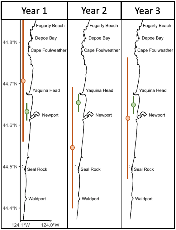
Over eight years of field work for the GRANITE project, consisting of over 40,000 km2 of ocean surveyed with 2,169 sightings of gray whales, our observations lead us to hypothesize that there are two broad space use strategies that whales use to optimize how they find enough prey to meet their energetic needs. For the moment, we are calling these strategies ‘home-body’ and ‘roamer’. As the name implies, a home-body is an individual that stays in a relatively small area and searches for food in this area consistently through time. A roamer, on the other hand, is an individual that travels and searches over a greater spatial area to find good pockets of food and does not generally tend to stay in just one place. In other words, we except a home-body to have a consistent activity center through time and a small activity range, while a roamer will have a much larger activity range and its activity center may vary more throughout the years (Figure 2).
Figure 2. Schematic representing one of the hypotheses we will be testing with our Bayesian spatial capture-recapture models. The schematic shows the activity centers (the circles) and activity ranges (vertical lines attached to the circles) of two individuals (green and orange) across three years in our central Oregon study area. The green individual represents our hypothesized idea of a home-body, whereas the orange individuals represents our idea of a roamer.
While this hypothesis sounds straightforward, there are a lot of decisions that I need to make in the Bayesian modeling process that can ultimately impact the results. For example, do all home-bodies in a population have the same size activity range or can the size vary between different home-bodies? If it can vary, by how much can it vary? These same questions apply for the roamers too. I have a long list of questions just like these, which means a lot of decision-making on my part, and that long list of hypotheses I previously mentioned. Luckily, I have a fantastic team made up of Leigh, committee members, and GRANITE collaborators that are guiding me through this process. In just a few more months, I hope to reveal how PCFG individuals distribute themselves in space and time throughout our central Oregon study area, and hence describe their exposure to different stressors. Stay tuned!
Did you enjoy this blog? Want to learn more about marine life, research, and conservation? Subscribe to our blog and get a weekly message when we post a new blog. Just add your name and email into the subscribe box below.
References
Borchers DL, Efford MG (2008) Spatially explicit maximum likelihood methods for capture-recapture studies. Biometrics 64:377-385.
Efford M (2004) Density estimation in live-trapping studies. Oikos 106:598-610.
Erlinge S, Sandell M (1986) Seasonal changes in the social organization of male stoats, Mustela erminea: An effect of shifts between two decisive resources. Oikos 47:57-62.
Gray TNE (2018) Monitoring tropical forest ungulates using camera-trap data. Journal of Zoology 305:173-179.
Pirotta E, Booth CG, Costa DP, Fleishman E, Kraus SD, and others (2018) Understanding the population consequences of disturbance. Ecology and Evolution 8(19):9934–9946.Royle J, Nichols J, Karanth KU, Gopalaswamy AM (2009) A hierarchical model for estimating density in camera-trap studies. Journal of Applied Ecology 46:118-127.
With the changing of the season, gray whales are starting their southbound migration that will end in the lagoons off the Baja California Mexico. The migration of the gray whale is the longest migration of any mammal—the round trip totals ~10,000 miles (Pike, 1962)!
Like these gray whales, I am also undertaking my own “migration” as I leave Newport to start my post-Master’s journey. However, my migration will be a little shorter than the gray whale’s journey—only ~3,000 miles—as I head back to the east coast. As I talked about in my previous blog, I have finished my thesis studying the energetics of gray whale foraging behaviors and I attended my commencement ceremony at the University of British Columbia last Wednesday. As my time with the GEMM Lab comes to a close, I want to take some time to reflect on my time in Newport.
Me in my graduation regalia (right) and my co-supervisor Andrew Trites holding the university mace (left) after my commencement ceremony at the University of British Columbia rose garden.
Many depictions of scientists show them working in isolation but in my time with the GEMM Lab I got to fully experience the collaborative nature of science. My thesis was a part of the GEMM Lab’s Gray whale Response to Ambient Noise Informed by Technology and Ecology (GRANITE) project and I worked closely with the GRANITE team to help achieve the project’s research goals. The GRANITE team has annual meetings where team members give updates on their contributions to the project and flush out ideas in a series of very busy days. I found these collaborative meetings very helpful to ensure that I was keeping the big picture of the gray whale study system in mind while working with the energetics data I explored for my thesis. The collaborative nature of the GRANITE project provided the opportunity to learn from people that have a different skill set from my own and expose me to many different types of analysis.
GRANITE team members hard at work thinking about gray whales and their physiological response to noise.
This summer I also was able to participate in outreach with the partnership of the Oregon State University Marine Mammal Institute and the Eugene Exploding Whales (the alternate identity of the Eugene Emeralds) minor league baseball team to promote the Oregon Gray Whale License plates. It was exciting to talk to baseball fans about marine mammals and be able to demonstrate that the Gray Whale License plate sales are truly making a difference for the gray whales off the Oregon coast. In fact, the minimally invasive suction cup tags used in to collect the data I analyzed in my thesis were funded by the OSU Gray Whale License plate fund!
Photo of the GEMM Lab promoting Oregon Gray Whale License plates at the Eugene Exploding Whales baseball game. If you haven’t already, be sure to “Put a whale on your tail!” to help support marine mammal research off the Oregon Coast.
Outside of the amazing science opportunities, I have thoroughly enjoyed the privilege of exploring Newport and the Oregon coast. I was lucky enough to find lots of agates and enjoyed consistently spotting gray whale blows on my many beach walks. I experienced so many breathtaking views from hikes (God’s thumb was my personal favorite). I got to attend an Oregon State Beavers football game where we crushed Stanford! And most of all, I am so thankful for all the friends I’ve made in my time here. These warm memories, and the knowledge that I can always come back, will help make it a little easier to start my migration away from Newport.
Me and my friends outside of Reser Stadium for the Oregon State Beavers football game vs Stanford this season. Go Beavs!!!
Me and my friends celebrating after my defense.
Did you enjoy this blog? Want to learn more about marine life, research, and conservation? Subscribe to our blog and get a weekly message when we post a new blog. Just add your name and email into the subscribe box below
References
Pike, G. C. (1962). Migration and feeding of the gray whale (Eschrichtius gibbosus). Journal of the Fisheries Research Board of Canada, 19(5), 815–838. https://doi.org/10.1139/f62-051
As you may remember, last year’s field season was a remarkable summer for our team. We were pleasantly surprised to find an increased number of whales in our study area compared to previous years and were even more excited that many of them were old friends. As we started this field season, we were all curious to know if this year would be a repeat. And it’s my pleasure to report that this season was even better!
Team selfies on the water
We started the season with an exciting day (6 known whales! see Lisa’s blog) and the excitement (and whales) just kept coming. This season we saw 71 individual whales across 215 sightings! Of those 71, 44 were whales we saw last year, and 10 were new to our catalog, meaning that we saw 17 whales this season that we had not seen in at least two years! There is something extra special about seeing a whale we have not seen in a while because it means that they are still alive, and the sighting gives us valuable data to continue studying health and survival. Another cool note is that 7 of our 12 new whales from last year came back this year, indicating recruitment to our study region.
Included in that group of 7 whales are the two calves from last year! Again, indicating good recruitment of new whales to our study area. We saw both Lunita and Manta (previously nick-named ‘Roly-poly’) throughout this season and we were always happy to see them back in our area and feeding on their own.
Drone image of Lunita from 2023
Drone image of Manta from 2023
We had an especially remarkable encounter with Lunita at the end of this season when we found this whale surface feeding on porcelain crab larvae (video 1)! This is a behavior that we rarely observe, and we’ve never seen a juvenile whale use this behavior before, inspiring questions around how Lunita knew how to perform this behavior.
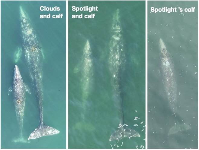
Not only did we resight our one-year-old friends, but we found two new calves born to well-known mature females (Clouds and Spotlight). We had previously documented Clouds with a calf (Cheetah) in 2016 so it was exciting to see her with a new calf and to meet Cheetah’s sibling! Cheetah has become one of our regulars so we’re curious to see if this new calf joins the regular crew as well. We’re also hoping that Spotlight’s calf will stick around; and we’re optimistic since we observed it feeding alone later in the season.
Collage of new calves from 2023! Left: Clouds and her calf, Center: Spotlight and her calf, Right: Spotlight’s calf independently foraging
Of course, 71 whales means heaps of data! We spent 226 hours on the water, conducted 132 drone flights (a record!), and collected 61 fecal samples! Those 132 flights were over 64 individual whales, with Casper and Pacman tying for “best whale to fly over” with 10 flights each. We collected 61 fecal samples from 26 individual whales with a three-way tie for “best pooper” between Hummingbird, Scarlett, and Zorro with 6 fecal samples each. And we continued to collect valuable prey and habitat data through 80 GoPro drops and 79 zooplankton net tows.
Above: (left) drone image of the team on our boat next to Pacman, (right) KC piloting the drone. Below: the team celebrating good fecal samples!
And if you were about to ask, “but what about tagging?!”, fear not! We continued our suction cup tagging effort with a successful window in July where we were joined by collaborators John Calambokidis from Cascadia Research Collective and Dave Cade from Hopkins Marine Station and deployed four suction-cup tags.
The team during our tagging effort this season.
It’s hard to believe all the work we’ve accomplished in the past five months, and I continue to be honored and proud to be on this incredible team. But as this season has come to a close, I have found myself reflecting on something else. Learning. Over the past several years we have learned so much about not only these whales in our study system but about how to conduct field work. And while learning is continuous, this season in particular has felt like an exciting time for both. In the past year our group has published work showing that we can detect pregnancy in gray whales using fecal samples and drone imagery (Fernandez Ajó et al., 2023), that PCFG gray whales are shorter and smaller than ENP whales (Bierlich et al., 2023), and that gray whales are consuming high levels of microplastics (Torres et al., 2023). We also have several manuscripts in review focused on our behavior work from drones and tags. While this information does not directly affect our field work, it does mean that while we’re observing these whales live, we better understand what we’re observing and we can come up with more specific, in-depth questions based on this foundation of knowledge that we’re building. I have enjoyed seeing our questions evolve each year based on our increasing knowledge and I know that our collaborative, inquisitive chats on the boat will only continue inspiring more exciting research.
On top of our gray whale knowledge, we have also learned so much about field work. When I think back to the early days compared to now, there is a stark difference in our knowledge and our confidence. We do a lot on our little boat! And so many steps that we once relied on written lists to remember to do are now just engrained in our minds and bodies. From loading the boat, to setting up at the dock, to the go pro drops, fecal collections, drone operations, photo taking, and photo ID, our team has become quite the well-oiled machine. We were also given the opportunity to reflect on everything we’ve learned over the past years when it was our turn to train our new team member, Nat! Nat is a new PhD student in the GEMM lab who is joining team GRANITE. Teaching her all the ins and outs of our fieldwork really emphasized how much we ourselves have learned.
Nat’s first days in the field!
On a personal note, this was my third season as a drone pilot, and honestly, I was pleasantly surprised by my experience this season. Since I started piloting, I have experienced pretty intense nerves every time I’ve flown the drone. From stress dreams, to mild nausea, and an elevated heart rate, flying the drone was something that I didn’t necessarily look forward to. Don’t get me wrong – it’s incredibly valuable data and a privilege to watch the whales from a bird’s eye view in real time. But the responsibility of collecting good data, while keeping the drone and my team members safe was something that I felt viscerally. And while I gained confidence with every flight, the nerves were still as present as ever and I was starting to accept that I would never be totally comfortable as a pilot. Until this season, when the nerves finally cleared, and piloting became as innate as all the other field work components. While there are still some stressful moments, the nerves don’t come roaring back. I have finally gone through enough stressful situations to not be fazed by new ones. And while I am fully aware that this is just how learning works, I write this reflection as a reminder to myself and anyone going through the process of learning any new skill to push through that fear. Remember there can be a disconnect between the time when you know how to do something well, or well-enough, and the time when you feel comfortable doing it. I am just as proud of myself for persevering as I am of the team for collecting so much incredible data. And as I look ahead to my next scary challenge (finishing my PhD!), this is a feeling that I am trying to hold on to.
Stay tuned for updates from team GRANITE!
Did you enjoy this blog? Want to learn more about marine life, research, and conservation? Subscribe to our blog and get a weekly alert when we make a new post! Just add your name into the subscribe box below!
References
Bierlich, K. C., Kane, A., Hildebrand, L., Bird, C. N., Fernandez Ajo, A., Stewart, J. D., Hewitt, J., Hildebrand, I., Sumich, J., & Torres, L. G. (2023). Downsized: Gray whales using an alternative foraging ground have smaller morphology. Biology Letters, 19(8), 20230043. https://doi.org/10.1098/rsbl.2023.0043
Fernandez Ajó, A., Pirotta, E., Bierlich, K. C., Hildebrand, L., Bird, C. N., Hunt, K. E., Buck, C. L., New, L., Dillon, D., & Torres, L. G. (2023). Assessment of a non-invasive approach to pregnancy diagnosis in gray whales through drone-based photogrammetry and faecal hormone analysis. Royal Society Open Science, 10(7), 230452. https://doi.org/10.1098/rsos.230452
Torres, L. G., Brander, S. M., Parker, J. I., Bloom, E. M., Norman, R., Van Brocklin, J. E., Lasdin, K. S., & Hildebrand, L. (2023). Zoop to poop: Assessment of microparticle loads in gray whale zooplankton prey and fecal matter reveal high daily consumption rates. Frontiers in Marine Science, 10. https://www.frontiersin.org/articles/10.3389/fmars.2023.1201078
The winds are consistently (and sometimes aggressively) blowing from the north here on the Oregon coast, which can only mean one thing – summer has arrived! Since mid-May, the GRANITE (Gray whale Response to Ambient Noise Informed by Technology and Ecology) team has been looking for good weather windows to survey for gray whales and we have managed to get five great field work days already. In today’s blog post, I am going to share what (and who) we have seen so far.
On our first day of the field season, PI Leigh Torres, postdoc KC Bierlich and myself, were joined by a special guest: Dr. Andy Read. Andy is the director of the Duke University Marine Lab, where he also runs his own lab, which focuses on conservation biology and ecology of marine vertebrates. Andy was visiting the Hatfield Marine Science Center as part of the Lavern Weber Visiting Scientist program and was hosted here by Leigh. For those of you that do not know, Andy was Leigh’s graduate school advisor at Duke where she completed her Master’s and doctoral degrees. It felt very special to have Andy on board our RHIB Ruby for the day and to introduce him to some friends of ours. The first whale we encountered that day was “Pacman”. While we are always excited to re-sight an individual that we know, this sighting was especially mind-blowing given the fact that Leigh had “just” seen Pacman approximately two months earlier in Guerrero Negro, one of the gray whale breeding lagoons in Mexico (read this blog about Leigh and Clara’s pilot project there). Aside from Pacman, we saw five other individuals, all of which we had seen during last year’s field season.
The first day of field work for the 2023 GRANITE field season! From left to right: Leigh Torres, Lisa Hildebrand, Andy Read, and KC Bierlich. Source: L. Torres.
Since that first day on the water, we have conducted field work on four additional days and so far, we have only encountered known individuals in our catalog. This fact is exciting because it highlights the strong site fidelity that Pacific Coast Feeding Group (PCFG) gray whales have to areas within their feeding range. In fact, I am examining the residency and space use of each individual whale we have observed in our GRANITE study for one of my PhD chapters to better understand the level of fidelity individuals have to the central Oregon coast. Furthermore, this site fidelity underpins the unique, replicate data set on individual gray whale health and ecology that the GRANITE project has been able to progressively build over the years. So far during this field season in 2023, we have seen 13 unique individuals, flown the drone over 10 of them and collected four fecal samples from two, which represent critical data points from early on in the feeding season.
Our sightings this year have not only highlighted the high site fidelity of whales to our study area but have also demonstrated the potential for internal recruitment of calves born to “PCFG mothers” into the PCFG. Recruitment to a population can occur in two ways: externally (individuals immigrate into a population from another population) or internally (calves born to females that are part of the population return to, or stay, within their mothers’ population). Three of the whales we have seen so far this year are documented calves from females that are known to consistently use the PCFG range, including our central Oregon coast study area. In fact, we documented one of these calves, “Lunita”, just last year with her mother (see Clara’s recap of the 2022 field season blog for more about Lunita). The average calf survival estimate between 1997-2017 for the PCFG was 0.55 (Calambokidis et al. 2019), though it varied annually and widely (range: 0.34-0.94). Considering that there have been years with calf survival estimates as low as ~30%, it is therefore all the more exciting when we re-sight a documented calf, alive and well!
“Lunita”, an example of successful internal recruitment
We have also been collecting data on the habitat and prey in our study system by deploying our paired GoPro/RBR sensor system. We use the GoPro to monitor the benthic substrate type and relative prey densities in areas where whales are feeding. The RBR sensor collects high-frequency, in-situ dissolved oxygen and temperature data, enabling us to relate environmental metrics to relative prey measurements. Furthermore, we also collect zooplankton samples with a net to assess prey community and quality. On our five field work days this year, we have predominantly collected mysid shrimp, including gravid (a.k.a. pregnant) individuals, however we have also caught some Dungeness and porcelain crab larvae. The GEMM Lab is also continuing our collaboration with Dr. Susanne Brander’s lab at OSU and her PhD student Lauren Kashiwabara, who plan on conducting microplastic lab experiments on wild-caught mysid shrimp. Their plan is to investigate the growth rates of mysid shrimp under different temperature, dissolved oxygen, and microplastic load conditions. However, before they can begin their experiments, they need to successfully culture the mysids in the lab, which is why we collect samples for them to use as their ‘starter culture’. Stay tuned to hear more about this project as it develops!
So, all in all, it has been an incredibly successful start to our field season, marked by the return of many familiar flukes and flanks! We are excited to continue collecting rock solid GRANITE data this summer to increase our efforts to understand gray whale ecology and physiology.
References
Calambokidis, J., Laake, J., and Perez, A. (2019). Updated analyses of abundance and population structure of seasonal gray whales in the Pacific Northwest, 1996-2017. IWC, SC/A17/GW/05 for the Workshop on the Status of North Pacific Gray Whales. La Jolla: IWC.
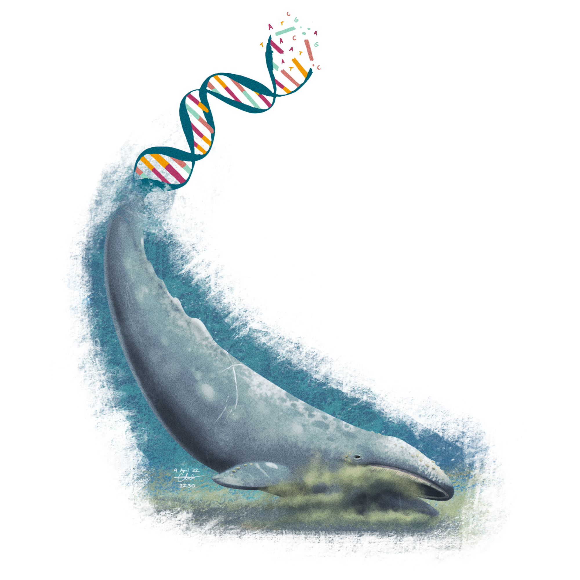
By Charles Nye, graduate student, OSU Department of Fisheries, Wildlife, & Conservation Sciences, Cetacean Conservation and Genomics Laboratory
Figure 1: An illustration (by me) of a feeding gray whale whose caudal end transitions into a DNA double helix.
Let’s consider how much stuff organisms shed daily. If you walk down a hallway, you’ll leave a microscopic trail of skin cells, evaporated sweat, and even more material if you so happen to sneeze or cough (as we’ve all learned). The residency of these bits and pieces in a given environment is on the order of days, give or take (Collins et al. 2018). These days, we can extract, amplify, and sequence DNA from leftover organismal material in environments (environmental DNA; eDNA), stomach contents (dietary DNA, dDNA), and other sources (Sousa et al. 2019; Chavez et al. 2021).
You might be familiar with genetic barcoding, where scientists are able to use documented and annotated pieces of a genome to identify a piece of DNA down to a species. Think of these as genetic fingerprints from a crime scene where all (described) species on Earth are prime suspects. With advancements in computing technology, we can barcode many species at the same time—a process known as metabarcoding. In short, you can now do an ecosystem-wide biodiversity survey without even needing to see your species of interest (Ficetola et al. 2008; Chavez et al. 2021).
(Before you ask: yes, people have tried sampling Loch Ness and came up with not a single strand of plesiosaur DNA (University of Otago, 2019).)
I received my crash course on metabarcoding when I was employed at the Monterey Bay Aquarium Research Institute (MBARI), right before grad school. There, I was employed to help refine eDNA survey field and laboratory methods (in addition to some cool robot stuff). Here at OSU, I use metabarcoding to research whale ecology, detection, and even a little bit of forensics work. Cetacean species (or evidence thereof) I’ve worked on include North Atlantic right whales (Eubalaena glacialis), killer whales (Orcinus spp.), and gray whales (Eschrichtius robustus).
Long-time readers of the GEMM Lab Blog are probably quite knowledgeable about the summertime grays—the Pacific Coast Feeding Group (PCFG). All of us here at OSU’s Marine Mammal Institute (MMI) are keenly interested in understanding why these whales hang out in the Pacific Northwest during the summer months and what sets them apart from the rest of the Eastern North Pacific gray whale population. What interests me? Well, I want to double-check what they’re eating—genetically.
“What does my study species eat?” is a straightforward but underappreciated question. It’s also deceptively difficult to address. What if your species live somewhere remote or relatively inaccessible? You can imagine this is a common logistical issue for most research in marine sciences. How many observations do you need to make to account for seasonal or annual changes in prey availability? Do all individuals in your study population eat the same thing? I certainly like to mix and match my diet.
Gray whale foraging ecology has been studied comprehensively over the last several decades, including an in-depth stomach content evaluation by Mary Nerini in 1984 and GEMMer Lisa Hildebrand’s MSc research. PCFG whales seem to prefer shrimpy little creatures called mysids, along with Dungeness crab (Cancer magister) larvae, during their stay in the Pacific Northwest (PNW), most notably the mysid Neomysis rayii (Guerrero 1989; Hildebrand et al. 2021). Indeed, the average energetic values of common suspected prey species in PNW waters rival the caloric richness of Arctic amphipods (Hildebrand et al. 2021). However, despite our wealth of visual foraging observations, metabarcoding may add an additional layer of resolution. For example, the ocean sunfish (Mola mola) was believed to exclusively forage on gelatinous zooplankton, but a metabarcoding approach revealed a much higher diversity of prey items, including other bony fishes and arthropods (Sousa et al. 2016).
Given all this exposition, you may be wondering: “Charles—how do you intend on getting dDNA from gray whales? Are you going to cut them open?”
Figure 2: The battle station, a vacuum pump that I use to filter out all of the particulate matter from a gray whale dDNA sample. The filter is made of polycarbonate track etch material, which melts away in the DNA extraction process—quite handy, indeed!
No. I’m going to extract DNA from their poop.
Well, actually, I’ve been doing that for the last two years. My lab (Cetacean Conservation and Genomics Laboratory, CCGL) and GEMM Lab have been collaborating to make lemonade out of, er…whale poop. An archive of gray whale fecal samples (with ongoing collections every field season) originally collected for hormone analyses presented itself with new life—the genomics kind. In addition to community-level data, we are also able to recover informative DNA from the gray whales, including sex ID from “depositing” individuals, though the recovery rate isn’t perfect.
Because the GEMM Lab/MMI can non-invasively collect multiple samples from the same individuals over time, dDNA metabarcoding is a great way to repeatedly evaluate the diets of the PCFG, just shy of being at the right place at the right time with a GoPro or drone to witness a feeding event. While we can get stomach contents and even usable dDNA from a naturally deceased whale, those data may not be ideal. How representative a stranded whale is of the population is dependent on the cause of death; an emaciated or critically injured individual, for example, is a strong outlier.
Figure 3: Presence/absence of the top 10 most-common taxonomic Families observed in the PCFG gray whale dDNA dataset (n = 20, randomly selected). Filled-in dots indicate at least one genetic read associated with that Family, and empty dots indicate none. Note the prey taxa: mysids (Mysidae), krill (Euphausiidae), and olive snails (Olividae).
Here’s a snapshot of progress to date for this dDNA metabarcoding project. I pulled out twenty random samples from my much larger working dataset (n = 82) for illustrative purposes (and legibility). After some bioinformatic wizardry, we can use a presence/absence approach to get an empirical glimpse at what passes through a PCFG gray whale. While I am able to recover species-level information, using higher-level taxonomic rankings summarizes the dataset in a cleaner fashion (and also, not every identifiable sequence resolves to species).
The title of most commonly observed prey taxa belongs to our friends, the mysids (Mysidae). Surprisingly, crabs and amphipods are not as common in this dataset, instead losing to krill (Euphausiidae) and olive snails (Olividae). The latter has been found in association with gray whale foraging grounds but not documented in a prey study (Jenkinson 2001). We also get an appreciable amount of interference from non-prey taxa, most notably barnacles (Balanidae), with an honorable mention to hydrozoans (Clytiidae, Corynidae). While easy to dismiss as background environmental DNA, as gray whales do forage at the benthos, these taxa were physically present and identifiable in Nerini’s (1984) gray whale stomach content evaluation.
So—can we conclude that barnacles and hydrozoans are an important part of a gray whale’s diet, as much as mysids? From decades of previous observations, we might say…probably not. Gray whales are actively targeting patches of crabby, shrimpy zooplankton things, and even employ novel foraging strategies to do so (Newell & Cowles 2006; Torres et al. 2018). However, the sheer diversity of consumed species does present additional dimensionality to our understanding of gray whale ecology.
The whales are eating these ancillary organisms, whether they intend to or not, and this probably does influence population dynamics, recruitment, and succession in these nearshore benthic habitats. After all, the shallow pits that gray whales leave behind post-feeding provide a commensal trophic link with other predatory taxa, including seabirds and groundfish (Oliver & Slattery 1985). Perhaps the consumption of these collateral species affects gray whale energetics and reflects on their “performance”?
I hope to address all of this and more in some capacity with my published work and graduate chapters. I’m confident to declare that we can document diet composition of PCFG whales using dDNA metabarcoding, but what comes next is where one can get lost in the sea(weeds). How does the diet of individuals compare to one another? What about at differing time points? Age groups? How many calories are in a barnacle? No need to fret—this is where the fun begins!
References
Chavez F, Min M, Pitz K, Truelove N, Baker J, LaScala-Grunewald D, Blum M, Walz K,
Nye C, Djurhuus A, et al. 2021. Observing Life in the Sea Using Environmental
DNA Oceanog. 34(2):102–119. doi:10.5670/oceanog.2021.218.
By Morgan O’Rourke-Liggett, Master’s Student, Oregon State University, Department of Fisheries, Wildlife, and Conservation Sciences, Geospatial Ecology of Marine Megafauna Lab
Avid readers of the GEMM Lab blog and other scientists are familiar with the incredible amounts of data collected in the field and the informative figures displayed in our publications and posters. Some of the more time-consuming and tedious work hardly gets talked about because it’s the in-between stage of science and other fields. For this blog, I am highlighting some of the behind-the-scenes work that is the subject of my capstone project within the GRANITE project.
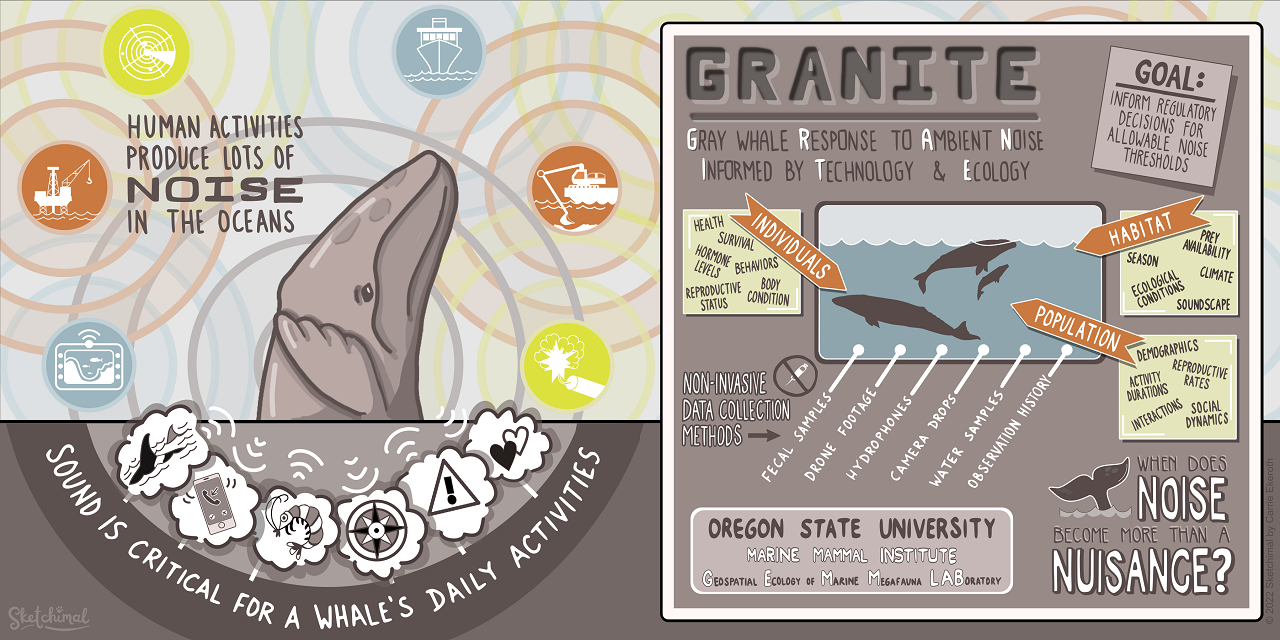
For those unfamiliar with the GRANITE project, this multifaceted and non-invasive research project evaluates how gray whales respond to chronic ambient and acute noise to inform regulatory decisions on noise thresholds (Figure 1). This project generates considerable data, often stored in separate Excel files. While this doesn’t immediately cause an issue, ongoing research projects like GRANITE and other long-term monitoring programs often need to refer to this data. Still, when scattered into separate long Excel files, it can make certain forms of analysis difficult and time-consuming. It requires considerable attention to detail, persistence, and acceptance of monotony. Today’s blog will dive into the not-so-glamorous side of science…data management and standardization!
Figure 1. Infographic for the GRANITE project. Credit: Carrie Ekeroth
Of the plethora of data collected from the GRANITE project, I work with the GPS trackline data from the R/V Ruby, environmental data recorded on the boat, gray whale sightings data, and survey summaries for each field day. These come to me as individual yearly spreadsheets, ranging from thirty entries to several thousand. The first goal with this data is to create a standardized survey effort conditions table. The second goal is to determine the survey distance from the trackline, using the visibility for each segment, and calculate the actual area surveyed for the segment and day. This blog doesn’t go into how the area is calculated. Still, all these steps are the foundation for finding that information so the survey area can be calculated.
The first step requires a quick run-through of the sighting data to ensure all dates are within the designated survey area by examining the sighting code. After the date is a three-letter code representing a different starting location for the survey, such as npo for Newport and dep for Depoe Bay. If any code doesn’t match the designated codes for the survey extent, those are hidden, so they are not used in the new table. From there, filling in the table begins (Figure 2).
Figure 2. A blank survey effort conditions table with each category listed at the top in bold.
Segments for each survey day were determined based on when the trackline data changed from transit to the sighting code (i.e., 190829_1 for August 29th, 2019, sighting 1). Transit indicated the research vessel was traveling along the coast, and crew members were surveying the area for whales. Each survey day’s GPS trackline and segment information were copied and saved into separate Excel workbook files. A specific R code would convert those files into NAD 1983 UTM Zone 10N northing and easting coordinates.
Those segments are uploaded into an ArcGIS database and mapped using the same UTM projection. The northing and easting points are imported into ArcGIS Pro as XY tables. Using various geoprocessing and editing tools, each segmented trackline for the day is created, and each line is split wherever there was trackline overlap or U shape in the trackline that causes the observation area to overlap. This splitting ensures the visibility buffer accounts for the overlap (Figure 3).
Figure 3. Segment 3 from 7/22/2019 with the visibility of 3 km portrayed as buffers. There are more than one because the trackline was split to account for the overlapping of the survey area. This approach accounts for the fact that this area where all three buffers overlap was surveyed 3 times.
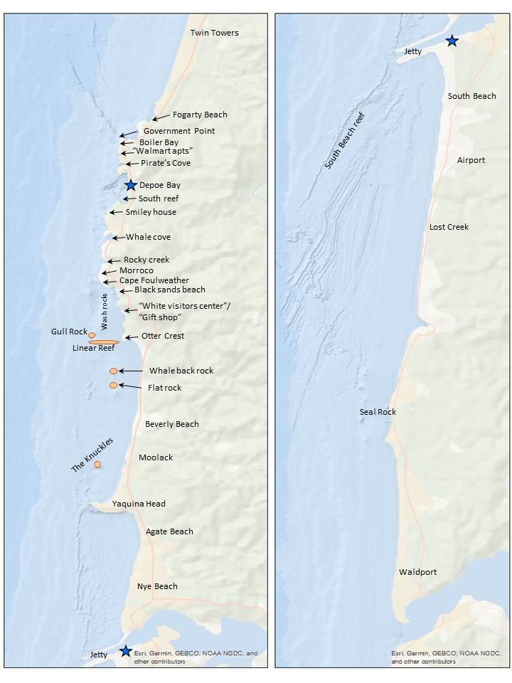
Once the segment lines are created in ArcGIS, the survey area map (Figure 4) is used alongside the ArcGIS display to determine the start and end locations. An essential part of the standardization process is using the annotated locations in Figure 4 instead of the names on the basemap for the location start and endpoints. This consistency with the survey area map is both for tracking the locations through time and for the crew on the research vessel to recognize the locations. The step assists with interpreting the survey notes for conditions at the different segments. The time starts and ends, and the latitude and longitude start and end are taken from the trackline data.
Figure 4. Map of the survey area with annotated locations (Created by L. Torres, GEMM Lab)
The sighting data includes the number of whales sighted, Beaufort Sea State, and swell height for the locations where whales were spotted. The environmental data from the sighting data is used as a guide when filling in the rest of the values along the trackline. When data, such as wind speed, swell height, or survey condition, is not explicitly given, matrices have been developed in collaboration with Dr. Leigh Torres to fill in the gaps in the data. These matrices and protocols for filling in the final conditions log are important tools for standardizing the environmental and condition data.
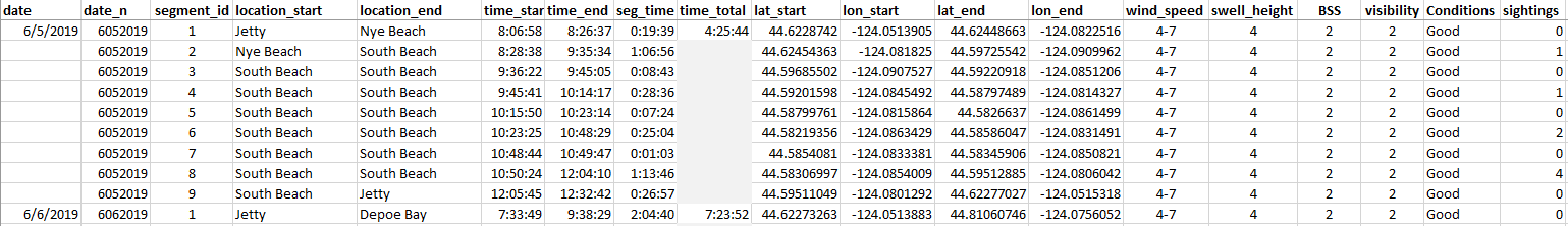
The final product for the survey conditions table is the output of all the code and matrices (Figure 5). The creation of this table will allow for accurate calculation of survey effort on each day, month, and year of the GRANITE project. This effort data is critical to evaluate trends in whale distribution, habitat use, and exposure to disturbances or threats.
Figure 5. A snippet of the completed 2019 season effort condition log.
The process of completing the table can be a very monotonous task, and there are several chances for the data to get misplaced or missed entirely. Attention to detail is a critical aspect of this project. Standardizing the GRANITE data is essential because it allows for consistency over the years and across platforms. In describing this aspect of my project, I mentioned three different computer programs using the same data. This behind-the-scenes work of creating and maintaining data standardization is critical for all projects, especially long-term research such as the GRANITE project.
Did you enjoy this blog? Want to learn more about marine life, research, and conservation? Subscribe to our blog and get a weekly message when we post a new blog. Just add your name and email into the subscribe box below.
Since its start, the GEMM Lab has been interested in the effect of vessel disturbance on whales. From former student Florence’s masters project to Leila’s PhD work, this research has shown that gray whales on their foraging grounds have a behavioral response to vessel presence (Sullivan & Torres, 2018) and a physiological response to vessel noise (Lemos et al., 2022). Presently, our GRANITE project is continuing to investigate the effect of ambient noise on gray whales, with an emphasis on understanding how these effects might scale up to impact the population as a whole (Image 1).
To date, all this work has been focused on gray whales feeding off the coast of Oregon, but I’m excited to share that this is about to change! In just a few weeks, Leigh and I will be heading south for a pilot study looking at the effects of whale watching vessels on gray whale mom/calf pairs in the nursing lagoons of Baja California, Mexico.
Image 1. Infographic for the GRANITE project. Credit: Carrie Ekeroth
We are collaborating with a Fernanda Urrutia Osorio, a PhD candidate at Scripps Institute of Oceanography, to spend a week conducting fieldwork in one of the nursing lagoons. For this project we will be collecting drone footage of mom/calf pairs in both the presence and absence of whale watching vessels. Our goal is to see if we detect any differences in behavior when there are vessels around versus when there are not. Tourism regulations only allow the whale watching vessels to be on the water during specific hours, so we are hoping to use this regulated pattern of vessel presence and absence as a sort of experiment.
Image 2. A mom and calf pair. NOAA/NMFS permit #21678.
The lagoons are a crucial place for mom/calf pairs, this is where calves nurse and grow before migration, and nursing is energetically costly for moms. So, it is important to study disturbance responses in this habitat since any change in behavior caused by vessels could affect both the calf’s energy intake and the mom’s energy expenditure. While this hasn’t yet been investigated for gray whales in the lagoons, similar studies have been carried out on other species in their nursing grounds.
Video 1. Footage of “likely nursing” behavior. NOAA/NMFS permit #21678.
We can use these past studies as blueprints for both data collection and processing. Disturbance studies such as these look for a wide variety of behavioral responses. These include (1) changes in activity budgets, meaning a change in the proportion of time spent in a behavior state, (2) changes in respiration rate, which would reflect a change in energy expenditure, (3) changes in path, which would indicate avoidance, (4) changes in inter-individual distance, and (5) changes in vocalizations. While it’s not necessarily possible to record all of these responses, a meta-analysis of research on the impact of whale watching vessels found that the most common responses were increases in the proportion of time spent travelling (a change in activity budget) and increased deviation in path, indicating an avoidance response (Senigaglia et al., 2016).
One of the key phrases in all these possible behavioral responses is “change in ___”. Without control data collected in the absence of whale watching vessels, it impossible to detect a difference. Some studies have conducted controlled exposures, using approaches with the research vessel as proxies for the whale watchers (Arranz et al., 2021; Sprogis et al., 2020), while others use the whale watching operators’ daily schedule and plan their data collection schedule around that (Sprogis et al., 2023). Just as ours will, all these studies collected data using drones to record whale behavior and made sure to collect footage before, during, and after exposure to the vessel(s).
One study focused on humpback mom/calf pairs found a decrease in the proportion of time spent resting and an increase in both respiration rate and swim speed during the exposure (Sprogis et al., 2020). Similarly, a study focused on short-finned pilot whale mom/calf pairs found a decrease in the mom’s resting time and the calf’s nursing time (Arranz et al., 2021). And, Sprogis et al.’s study of Southern right whales found a decrease in resting behavior after the exposure, suggesting that the vessels’ affect lasted past their departure (Sprogis et al., 2023, Image 3). It is interesting that while these studies found changes in different response metrics, a common trend is that all these changes suggest an increase in energy expenditure caused by the disturbance.
However, it is important to note that these studies focused on short term responses. Long term impacts have not been thoroughly estimated yet. These studies provide many valuable insights, not only into the response of whales to whale watching, but also a look at the various methods used. As we prepare for our fieldwork, it’s useful to learn how other researchers have approached similar projects.
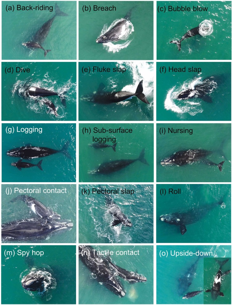
Image 3. Visual ethogram from Sprogis et al. 2023. This shows all the behaviors they identified from the footage.
I want to note that I don’t write this blog intending to condemn whale watching. I fully appreciate that offering the opportunity to view and interact with these incredible creatures is valuable. After all, it is one of the best parts of my job. But hopefully these disturbance studies can inform better regulations, such as minimum approach distances or maximum engine noise levels.
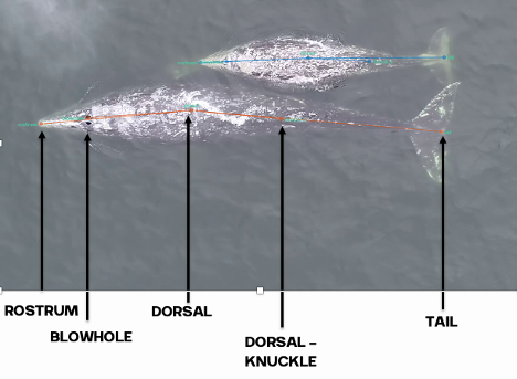
As these studies have done, our first step will be to establish an ethogram of behaviors (our list of defined behaviors that we will identify in the footage) using our pilot data. We can also record respiration and track line data. An additional response that I’m excited to add is the distance between the mom and her calf. Former GEMM Lab NSF REU intern Celest will be rejoining us to process the footage using the AI method she developed last summer (Image 4). As described in her blog, this method tracks a mom and calf pair across the video frames, and allows us to extract the distance between them. We look forward to adding this metric to the list and seeing what we can glean from the results.
Image 4. Example of a labelled frame from SLEAP, highlighting labels: rostrum, blowhole, dorsal, dorsal-knuckle, and tail. This labels are drawn to train the software to recognize the whales in unlabelled frames.
While we are just getting started, I am excited to see what we can learn about these whales and how best to study them. Stay tuned for updates from Baja!
Did you enjoy this blog? Want to learn more about marine life, research, and conservation? Subscribe to our blog and get a weekly alert when we make a new post! Just add your name into the subscribe box below!
References
Arranz, P., Glarou, M., & Sprogis, K. R. (2021). Decreased resting and nursing in short-finned pilot whales when exposed to louder petrol engine noise of a hybrid whale-watch vessel. Scientific Reports, 11(1), 21195. https://doi.org/10.1038/s41598-021-00487-0
Lemos, L. S., Haxel, J. H., Olsen, A., Burnett, J. D., Smith, A., Chandler, T. E., Nieukirk, S. L., Larson, S. E., Hunt, K. E., & Torres, L. G. (2022). Effects of vessel traffic and ocean noise on gray whale stress hormones. Scientific Reports, 12(1), Article 1. https://doi.org/10.1038/s41598-022-14510-5
Senigaglia, V., Christiansen, F., Bejder, L., Gendron, D., Lundquist, D., Noren, D., Schaffar, A., Smith, J., Williams, R., Martinez, E., Stockin, K., & Lusseau, D. (2016). Meta-analyses of whale-watching impact studies: Comparisons of cetacean responses to disturbance. Marine Ecology Progress Series, 542, 251–263. https://doi.org/10.3354/meps11497
Sprogis, K. R., Holman, D., Arranz, P., & Christiansen, F. (2023). Effects of whale-watching activities on southern right whales in Encounter Bay, South Australia. Marine Policy, 150, 105525. https://doi.org/10.1016/j.marpol.2023.105525
Sprogis, K. R., Videsen, S., & Madsen, P. T. (2020). Vessel noise levels drive behavioural responses of humpback whales with implications for whale-watching. ELife, 9, e56760. https://doi.org/10.7554/eLife.56760
Sullivan, F. A., & Torres, L. G. (2018). Assessment of vessel disturbance to gray whales to inform sustainable ecotourism. Journal of Wildlife Management, 82(5), 896–905. https://doi.org/10.1002/jwmg.21462
After my graduation, since I have tropical blood running in my veins, I literally crossed the entire country in search of blue and sunny skies, warm weather and ocean, and of course different opportunities to continue doing research involving stressors and physiological responses in marine mammals and other marine organisms. It didn’t take me long to start a position as a postdoctoral associate with the Institute of Environment at Florida International University. I have learned so much in these past two years while mainly working with toxicology and stress biomarkers in a wide range of marine individuals including corals, oysters, fish, dolphins, and now manatees. I have started a new chapter in my life, and I am very eager to see where it takes me.
Talking about chapters… my Ph.D. thesis comprised four different chapters and I had published only the first one when I left Oregon: “Intra- and inter-annual variation in gray whale body condition on a foraging ground”. In this study we used drone-based photogrammetry to measure and compare gray whale body condition along the Oregon coast over three consecutive foraging seasons (June to October, 2016-2018). We described variations across the different demographic units, improved body condition with the progression of feeding seasons, and variations across years, with a better condition in 2016 compared to the following two years. Then in 2020, I was able to publish my second chapter entitled “Assessment of fecal steroid and thyroid hormone metabolites in eastern North Pacific gray whales”. In this study, we used gray whale fecal samples to validate and quantify four different hormone metabolite concentrations (progestins, androgens, glucocorticoids, and thyroid hormone). We reported variation in progestins and androgens by demographic unit and by year. Almost a year later, my third chapter “Stressed and slim or relaxed and chubby? A simultaneous assessment of gray whale body condition and hormone variability” was published. In this chapter, we documented a negative correlation between body condition and glucocorticoids, meaning that slim whales were more stressed than the chubby ones.
These three chapters were “relatively easy” to publish compared to my fourth chapter, which had a long and somewhat stressful process (which is funny as I am trying to report stress responses in gray whales). Changes between journals, titles, analyses, content, and focus had to be made over the past year and a half for it to be accepted for publication. However, I believe that it was worth the extra work and invested time as our research definitely became more robust after all of the feedback provided by the reviewers. This chapter, now entitled “Effects of vessel traffic and ocean noise on gray whale stress hormones” was finally published earlier this month at the Nature Scientific Reports journal, and I’ll describe it further below.
Increased human activities in the last decades have altered the marine ecosystem, leaving us with a noisier, warmer, and more contaminated ocean. The noise caused by the dramatic increase in commercial and recreational shipping and vessel traffic1-3 has been associated with negative impacts on marine wildlife populations4,5. This is especially true for baleen whales, whose frequencies primarily used for communication, navigation, and foraging6,7 are “masked” by the noise generated by this watercraft. Several studies have reported alterations in marine mammal behavioral states8-11, increased group cohesion12-14, and displacement8,15 due to this disturbance, however, just a few studies have considered their physiological responses. Examples of physiological responses reported in marine mammals include altered metabolic rate15,16 and variations in stress-related hormone (i.e., glucocorticoids) concentrations relative to vessel abundance and ambient noise17,18. Based on this context and on the scarcity of such assessments, we attempted to determine the effects of vessel traffic and associated ambient noise, as well as potential confounding variables (i.e., body condition, age, sex, time), on gray whale fecal glucocorticoid concentrations.
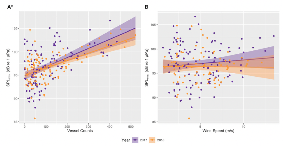
In addition to the data used in my previous three chapters collected from gray whales foraging off the Oregon coast, we also collected ambient noise levels using hydrophones, vessel count data from the Oregon Department of Fish and Wildlife (ODFW), and wind data from NOAA National Data Buoy Center (NDBC). Our first finding was a positive correlation between vessel counts and underwater noise levels (Fig. 1A), likely indicating that vessel traffic is the dominant source of noise in the area. To confirm this, we also compared underwater noise levels with wind speed (Fig. 1B), but no correlations were found.
Figure 1: Linear correlations between noise levels (daily median root mean square [rms] sound pressure level [SPL] in dB [re 1 μPa]; 50–1000 Hz) recorded on a hydrophone deployed outside the Newport harbor entrance during June to October of 2017 and 2018 and (A) vessel counts in Newport and Depoe Bay, Oregon, USA, and (B) daily median wind speed (m/s) from an anemometer station located on South Beach, Newport, Oregon, USA (station NWPO3). Asterisk indicates significant correlations between SPL and vessel counts in both years.
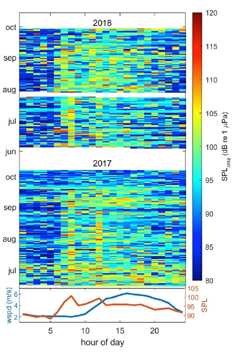
We also investigated noise levels by the hour of the day (Fig. 2), and we found that noise levels peaked between 6 and 8 am most days, coinciding with the peak of vessels leaving the harbor to get to fishing grounds. Another smaller peak is seen at 12 pm, which may represent “half-day fishing charter” vessels returning to the harbor. In contrast, wind speeds (in the lower graph) peaked between 3 and 4 pm, thus confirming the absence of correlation between noise and wind and providing more evidence that noise levels are dominated by the vessel activity in the area.
Figure 2: Median noise levels (root mean square sound pressure levels—SPLrms) for each hour of each day recorded on a hydrophone (50–10,000 Hz) deployed outside the Newport harbor entrance during June to October of 2017 (middle plot) and 2018 (upper plot), and hourly median noise level (SPL) against hourly median wind speed (lower plot) from an anemometer station located on South Beach, Newport, Oregon, USA (station NWPO3) over the same time period.
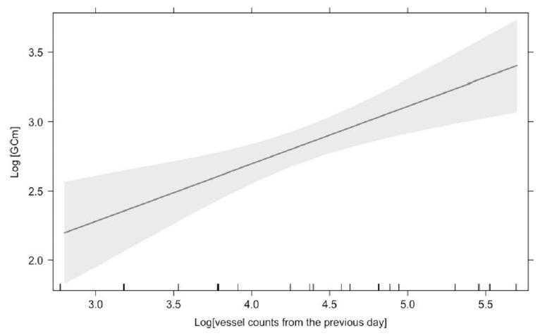
Finally, we assessed the effects of vessel counts, month, year, sex, whale body condition, and other hormone metabolites on glucocorticoid metabolite (GCm; “stress”) concentrations. Since we are working with fecal samples, we needed to consider the whale gut transit time and go back in time to link time of exposure (vessel counts) to response (glucocorticoid concentrations). However, due to uncertainty regarding gut transit time in baleen whales, we compared different time lags between vessel counts and fecal collection. The gut transit time in large mammals is ~12 hours to 4 days3,19,20, so we investigated the influence of vessel counts on whale “stress hormone levels” from the previous 1 to 7 days. The model with the most influential temporal scale included vessel counts from previous day, which showed a significant positive relationship with GCm (the “stress hormone level”) (Fig. 3).
Figure 3: The effect of vessel counts in Newport and Depoe Bay (Oregon, USA) on the day before fecal sample collection on gray whale fecal glucocorticoid metabolite (GCm) concentrations.
Thus, the “take home messages” of our study are:
The soundscape in our study area is dominated by vessel noise.
Vessel counts are strongly correlated with ambient noise levels in our study area.
Gray whale glucocorticoid levels are positively correlated with vessel counts from previous day meaning that gray whale gut transit time may occur within ~ 24 hours of the disturbance event.
These four chapters were all very important studies not only to advance the knowledge of gray whale and overall baleen whale physiology (as this group is one of the most poorly understood of all mammals given the difficulties in sample collection21), but also to investigate potential sources for the unusual mortality event that is currently happening (2019-present) to the Eastern North Pacific population of gray whales. Such studies can be used to guide future research and to inform population management and conservation efforts regarding minimizing the impact of anthropogenic stressors on whales.
I am very glad to be part of this project, to see such great fruits from our gray whale research, and to know that this project is still at full steam. The GEMM Lab continues to collect and analyze data for determining gray whale body condition and physiological responses in association with ambient noise (Granite, Amber and Diamond projects). The gray whales thank you for this!
Cited Literature
1. McDonald, M. A., Hildebrand, J. A. & Wiggins, S. M. Increases in deep ocean ambient noise in the Northeast Pacific west of San Nicolas Island, California. J. Acoust. Soc. Am. 120, 711–718 (2006).
2. Kaplan, M. B. & Solomon, S. A coming boom in commercial shipping? The potential for rapid growth of noise from commercial ships by 2030. Mar. Policy 73, 119–121 (2016).
3. McCarthy, E. International regulation of underwater sound: establishing rules and standards to address ocean noise pollution (Kluwer Academic Publishers, 2004).
4. Weilgart, L. S. The impacts of anthropogenic ocean noise on cetaceans and implications for management. Can. J. Zool. 85, 1091–1116 (2007).
5. Bas, A. A. et al. Marine vessels alter the behaviour of bottlenose dolphins Tursiops truncatus in the Istanbul Strait, Turkey. Endanger. Species Res. 34, 1–14 (2017).
6. Erbe, C., Reichmuth, C., Cunningham, K., Lucke, K. & Dooling, R. Communication masking in marine mammals: a review and research strategy. Mar. Pollut. Bull. 103, 15–38 (2016).
7. Erbe, C. et al. The effects of ship noise on marine mammals: a review. Front. Mar. Sci. 6 (2019).
8. Sullivan, F. A. & Torres, L. G. Assessment of vessel disturbance to gray whales to inform sustainable ecotourism. J. Wildl. Manag. 82, 896–905 (2018).
9. Pirotta, E., Merchant, N. D., Thompson, P. M., Barton, T. R. & Lusseau, D. Quantifying the effect of boat disturbance on bottlenose dolphin foraging activity. Biol. Conserv. 181, 82–89 (2015).
10. Dans, S. L., Degrati, M., Pedraza, S. N. & Crespo, E. A. Effects of tour boats on dolphin activity examined with sensitivity analysis of Markov chains. Conserv. Biol. 26, 708–716 (2012).
11. Christiansen, F., Rasmussen, M. & Lusseau, D. Whale watching disrupts feeding activities of minke whales on a feeding ground. Mar. Ecol. Prog. Ser. 478, 239–251 (2013).
12. Bejder, L., Samuels, A., Whitehead, H. & Gales, N. Interpreting short-term behavioural responses to disturbance within a longitudinal perspective. Anim. Behav. 72, 1149–1158 (2006).
13. Nowacek, S. M., Wells, R. S. & Solow, A. R. Short-term effects of boat traffic on Bottlenose dolphins, Tursiops truncatus, in Sarasota Bay, Florida. Mar. Mammal. Sci. 17, 673–688 (2001).
14. Bejder, L., Dawson, S. M. & Harraway, J. A. Responses by Hector’s dolphins to boats and swimmers in Porpoise Bay, New Zealand. Mar. Mammal Sci. 15, 738–750 (1999).
15. Lusseau, D. Male and female bottlenose dolphins Tursiops spp. have different strategies to avoid interactions with tour boats in Doubtful Sound. New Zealand. Mar. Ecol. Prog. Ser. 257, 267–274 (2003).
16. Sprogis, K. R., Videsen, S. & Madsen, P. T. Vessel noise levels drive behavioural responses of humpback whales with implications for whale-watching. Elife 9, e56760 (2020).
17. Ayres, K. L. et al. Distinguishing the impacts of inadequate prey and vessel traffic on an endangered killer whale (Orcinus orca) population. PLoS ONE 7, e36842 (2012).
18. Rolland, R. M. et al. Evidence that ship noise increases stress in right whales. Proc. R. Soc. B Biol. Sci. 279, 2363–2368 (2012).
19. Wasser, S. K. et al. A generalized fecal glucocorticoid assay for use in a diverse array of nondomestic mammalian and avian species. Gen. Comp. Endocrinol. 120, 260–275 (2000).
20. Hunt, K. E., Trites, A. W. & Wasser, S. K. Validation of a fecal glucocorticoid assay for Steller sea lions (Eumetopias jubatus). Physiol. Behav. 80, 595–601 (2004).
21. Hunt, K. E. et al. Overcoming the challenges of studying conservation physiology in large whales: a review of available methods. Conserv. Physiol. 1, cot006–cot006 (2013).