Alana Cary, St. Mary’s College of Maryland Undergraduate in Marine Science, 2026 NSF REU and GEMM Lab SAPPHIRE Project Intern
Hello everyone! My name is Alana Cary, and I was one of the NSF REU interns with the GEMM Lab this summer. I am currently in my senior year at St. Mary’s College of Maryland (SMCM), where I study Marine Science. Growing up along the Chesapeake Bay, I was always captivated by the connection between people and marine ecosystems. That curiosity led me to pursue marine mammal ecology, and this summer I had the amazing opportunity to travel across the country and dive into bioacoustics research with the GEMM Lab at Oregon State University’s Hatfield Marine Science Center.
My project, Daily Diel Ins: Investigating Diel and Seasonal Calling Patterns of New Zealand Blue Whales, explored how the world’s largest animals use sound over the course of the day and throughout the year. Working under the mentorship of Dawn Barlow and Leigh Torres, I spent ten weeks immersed in whale calls, coding, and a lot of matcha (shoutout to RISE cafe!).
Why study whale voices?
Blue whales (Balaenoptera musculus) are record-breakers: the largest animals to have ever lived, producers of the loudest biological sounds, and yet, surprisingly elusive. They spend most of their lives far beneath the surface, only surfacing briefly to breathe. This lifestyle makes them difficult to study visually. But blue whales leave behind something extremely powerful — their voices.
Baleen whales rely heavily on low-frequency sounds to forage, navigate, and communicate across vast distances (Clark & Ellison 2004). New Zealand blue whales are unique since they produce a distinct regional song (Torres et al. 2013; Barlow et al. 2018), and their calls provide insight into both foraging and reproductive behavior.
Blue whales produce two main call types (Figure 3):
- Songs – long, stereotyped sequences produced by males, likely used in reproduction and communication.
- D calls – short, frequency-modulated downsweeps produced by both sexes, often linked to foraging or social behavior.
Previous research has described the seasonal calling patterns of New Zealand blue whales (Barlow et al. 2023), but until now, diel (day–night) patterns had not been studied. This is important because blue whales’ primary prey, krill, perform diel vertical migration (DVM) in many parts of the ocean — ascending at night and descending during the day. If whale calls are tied to foraging or social interactions, they might vary depending on these light-driven prey movements.
Listening to giants: methods and workflow
My study focused on the South Taranaki Bight (STB), a productive upwelling region between New Zealand’s North and South Islands. The STB supports a unique population of blue whales year-round, providing foraging and reproductive opportunities (Torres et al. 2013; Barlow et al. 2018), but it is also an area with heavy human activity, including shipping, oil and gas, and fishing. Understanding when and how whales call here helps identify times of overlap with disturbance.
Here’s how I studied their voices:
- Hydrophones in the field – We used Rockhopper autonomous hydrophones, which are compact devices designed to record low-frequency sound for long periods (Klinck et al. 2020). These instruments collected a year of acoustic data in the STB (January 2024–January 2025).
- Manual annotation – From this massive dataset, one day was randomly selected from every two weeks (24 days total) and I manually annotated spectrograms of songs and D calls in Raven Pro. I identified songs in the 0–75 Hz band and D calls up to 150 Hz, following published criteria.
- Machine learning classification – These manual annotations were used to evaluate a BirdNET machine learning model (Kahl et al. 2021) trained to detect whale calls. The model then predicted calls across the entire year-long dataset.
- Validation – Because D calls are harder to classify, I manually reviewed all predicted D calls to remove false positives. Song detections, which had extremely high precision and recall, were kept without this extra step.
- Binning into diel phases – I aggregated call detections by hour and used the suncalc R package (Thieurmel et al. 2022) to assign diel phases (day or night). I also grouped calls by month and season to evaluate seasonal trends.
- Statistics in RStudio – To test whether month, diel phase, or their interaction influenced call rates, I ran two-way ANOVAs with post hoc Tukey’s HSD tests for pairwise comparisons
Results: different rhythms for different calls
The results revealed that songs and D calls follow very different patterns.
Songs – Seasonal, weakly diel:
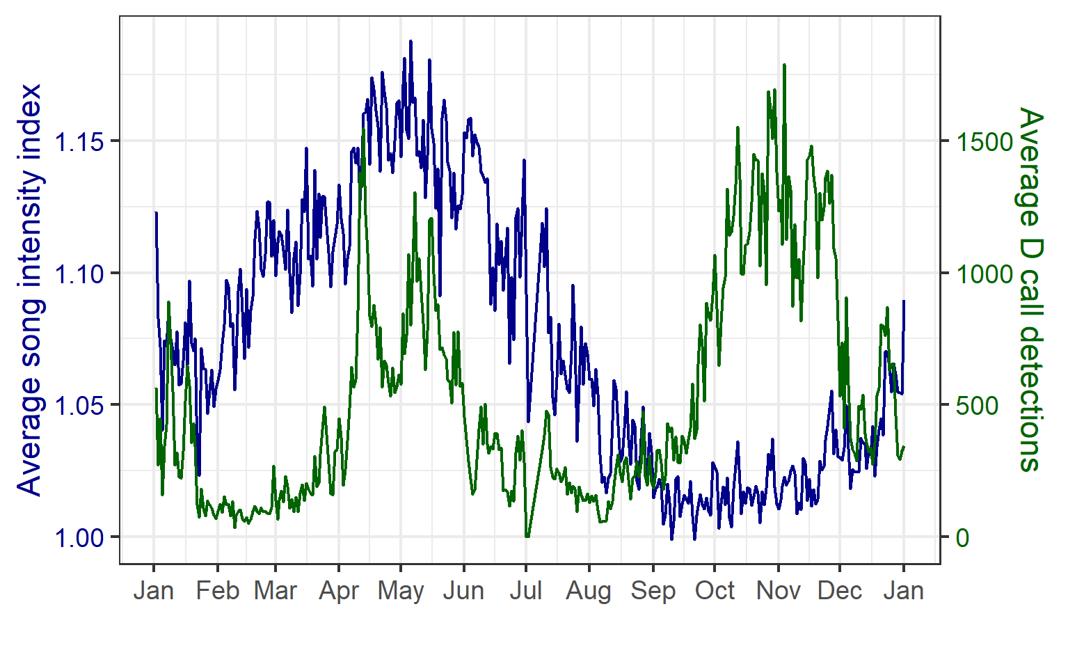
- Songs showed strong seasonal variation, peaking in late summer and autumn (February–May).
- Diel effects were weaker but significant: slightly more daytime calling, consistent across months.
- This suggests that songs are driven mainly by reproductive cycles, not daily light cues.
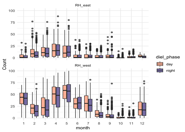
D calls – Both seasonal and diel:
- D calls showed highly significant effects of month, diel phase, and their interaction.
- Calling rates peaked in spring and summer, with more D calls during daytime hours.
- The diel effect varied by month: some months showed strong differences between day and night, while others showed none.
- This suggests that D calls track foraging, responding to increased krill availability during spring and summer months, and krill’s diel vertical migration
Why does this matter?
Understanding when whales call is more than an academic exercise. The South Taranaki Bight is not only an important whale habitat, it’s also a busy human space. By identifying when whales are most acoustically active, we can better understand potential conflicts with anthropogenic noise from shipping or industrial activities. For example, the fact that daytime D calls peak in spring and summer, times of high foraging effort, means that increased vessel noise during these periods could disrupt critical feeding-related communication. This kind of fine-scale temporal knowledge can inform management strategies to reduce human impacts on a vulnerable whale population. These insights also feed into the GEMM Lab’s SAPPHIRE project goal: linking oceanography, prey dynamics, physiology, and acoustics to understand how blue whales respond to a rapidly changing ocean (Barlow & Torres, 2021; Barlow et al., 2023).
Reflections on my REU journey
When I first arrived at Hatfield, I had never worked with passive acoustic data before. At first, spectrograms just looked like fuzzy TV static. But every day I learned to trust the process. Soon, I was able to fly through annotations and recognize calls without even seeing them on the spectrogram— just listening. I remember creating my plots and seeing the clear diel patterns, I couldn’t help but grin.
There were some moments that were frustrating as well, like when my entire selection table would delete and I’d have to start over, or debugging the same error message with no hope of figuring it out. But these frustrations taught me to be patient, persistent, and to not be afraid to ask for help. Weekly check-ins with Dawn pushed me to put my critical thinking to the test to decipher what my results meant. My co-interns and lab mates provided laughter, support, and encouragement that made the work even more rewarding. Beyond the data, I also learned how science is built on community. Research isn’t just all about running tests and analyzing plots, it’s about sharing ideas, collaboration, and building on each other’s work.
As a first-generation college student, this opportunity showed me that I can belong in marine science. I leave this summer with new skills in bioacoustics, statistics, and science communication, but also with a deeper sense of confidence and belonging in research.
Did you enjoy this blog? Want to learn more about marine life, research, and conservation? Subscribe to our blog and get a weekly alert when we make a new post! Just add your name into the subscribe box below!
References
Barlow, D. R., Klinck, H., Ponirakis, D., Branch, T. A., & Torres, L. G. (2023). Environmental conditions and marine heatwaves influence blue whale foraging and reproductive effort. Ecology and Evolution, 13(2), e9770. https://doi.org/10.1002/ece3.9770
Barlow, D. R., & Torres, L. G. (2021). Planning ahead: Dynamic models forecast blue whale distribution with applications for spatial management. Journal of Applied Ecology, 58(11), 2493–2504. https://doi.org/10.1111/1365-2664.13992
Barlow, D. R., Torres, L. G., Hodge, K. B., Steel, D., Baker, C. S., Chandler, T. E., Bott, N., Constantine, R., Double, M. C., Gill, P., Glasgow, D., Hamner, R. M., Lilley, C., Ogle, M., Olson, P. A., Peters, C., Stockin, K. A., Tessaglia-Hymes, C. T., & Klinck, H. (2018). Documentation of a New Zealand blue whale population based on multiple lines of evidence. Endangered Species Research, 36, 27–40. https://doi.org/10.3354/esr00891
Clark, C. W., & Ellison, W. T. (2004). Potential use of low-frequency sounds by baleen whales for probing the environment: Evidence from models and empirical measurements. In Echolocation in Bats and Dolphins (Vol. 1–1, pp. 564–589). Univeristy of Chicago Press.
Kahl, S., Wood, C. M., Eibl, M., & Klinck, H. (2021). BirdNET: A deep learning solution for avian diversity monitoring. Ecological Informatics, 61, 101236. https://doi.org/10.1016/j.ecoinf.2021.101236
Klinck, H., Winiarski, D., Mack, R. C., Tessaglia-Hymes, C. T., Ponirakis, D. W., Dugan, P. J., Jones, C., & Matsumoto, H. (2020). The Rockhopper: A compact and extensible marine autonomous passive acoustic recording system. Global Oceans 2020: Singapore – U.S. Gulf Coast, 1–7. https://doi.org/10.1109/IEEECONF38699.2020.9388970
Thieurmel, B., & Elmarhraoui, A. (2022). suncalc: Compute sun position, sunlight phases, moon position and lunar phase (Version 0.5.1) [R package]. Comprehensive R Archive Network (CRAN). https://CRAN.R-project.org/package=suncalc
Torres, L. (2013). Evidence for an unrecognised blue whale foraging ground in New Zealand. New Zealand Journal of Marine and Freshwater Research, 47(2), 235–248. https://doi.org/10.1080/00288330.2013.773919