Every breath [a whale] takes: How and why we study cetacean respiration

Clara Bird, PhD Candidate, OSU Department of Fisheries, Wildlife, and Conservation Sciences, Geospatial Ecology of Marine Megafauna Lab

We need energy to function and survive. For animals in the wild who may have limited food availability, knowing how they spend their energy is a critical question for many scientists because it fundamentally informs how we understand their decisions about where they go and what they do. The entire field of foraging theory is founded on the concept that animals optimize their ratio of energy in and energy out so that they have enough energy to survive, reproduce (pass on their genes), watch out for threats, if need be, and rest. And, if we understand an animal’s ‘typical’ energy budget, we can then try to predict how disturbance or environmental change will affect their actual energy budgets as a consequence of that change. But how do we measure energy expenditure?

The most commonly measured energy currency is oxygen. Since our cells use oxygen to produce energy (this is why we need oxygen to live), we can measure oxygen consumption as a metric of energy expenditure. The more oxygen we consume, the more energy we’re expending. In ideal lab settings, oxygen consumption can be accurately measured by placing the subject in a chamber where the oxygen flow can be controlled (Speakman, 1999). However, you can probably see how that approach is problematic for measuring oxygen consumption in most large free-living animals, especially cetaceans. It isn’t exactly feasible to put a whale in a box.

Image 1. A great tit in a metabolic chamber. Figure 1 from Broggi et al., 2009

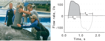
Fortunately, a tool called a spirometer was developed to measure oxygen consumption in restrained cetaceans. A spirometer is a device that can be placed over the blowhole(s) of an individual to accurately measure the amount of air that is exhaled and inhaled (Figure 1).  For trained cetaceans in captivity (e.g., dolphins), spirometers can be used to quantify how respiration changes after the animal performs certain behaviors (Fahlman et al., 2019). The breathing patterns of diving mammals are particularly interesting because they cannot breathe during most of their exercise (energy expenditure) as they are underwater. So, their breathing patterns after a dive tell us a lot about how much energy they spent during that dive. For example, Fahlman et al. (2019) used spirometer data from dolphins in captivity to study how their breathing patterns changed while recovering from dives of different durations. Interestingly, they found that after longer dives, dolphins took larger breaths (i.e., inhaled more air) while recovering but did not change the number of breaths. This finding is particularly relevant to the work we are conducting in the GEMM lab, where we utilize breathing patterns to quantify the energy expenditure of cetaceans in the wild, where spirometers cannot be used.

Figure 1. Figure 1 from Sumich et al. (2023). Left: a spirometer being held over the blow holes of JJ, a gray whale calf at sea world in 1997; one of the rare times that a large baleen whale was in captivity and available for these measurements. Right: example of a plot created using the data from a spirometer over JJ’s blow holes. The duration of a “blow” (exhale followed by immediate inhale) is on the x-axis, the flow rate (in liters per second) is on the y-axis. The positive curve during the exhale shows that the whale strongly exhales a lot of air very quickly, then the negative curve shows the whale inhaling a lot of air very quickly.

In a previous blog, I described how inter-breath intervals (the time between consecutive blows) are useful for estimating energy expenditure in free-living cetaceans. Essentially, a shorter interval indicates that the whale was just engaged in an energetically demanding activity. When you’re recovering from a sprint, you breathe faster (i.e., with shorter inter-breath intervals), than when you’re recovering from a walk. However, a big assumption in using inter-breath intervals as a proxy for energy expenditure is that every breath is equal. But as Fahlman et al. emphasize in their 2016 paper, every blow is not equal (Fahlman et al., 2016). In addition to varying the time between breaths, an animal can vary the intensity of each breath (e.g., Fahlman et al., 2019), the duration of each breath (Sumich et al., 2023), the number of breaths, and even the expansion of their nostrils (Nazario et al., 2022; check out this blog for more).

Image 2. Gray whale blow. Source: https://www.lajollalight.com/sdljl-natural-la-jolla-winter-wildlife-2015jan08-story.html

Altogether, this means that it’s important to measure every breath and that no one metric tells the complete story. This also means my research question focused on comparing the energetic costs of different tactics is more complicated than I originally thought. If we go back to the first blog I wrote on this topic, I was planning ons only using inter-breath intervals to estimate energy expenditure. Fast forward four years, with all my new knowledge gained on respiration variability, I’ve modified my plan and now I’m working to first understand how all these different metrics of breathing relate to each other. Then, I’ll compare how breathing varies between different foraging tactics, which is an important follow up to my questions around individual specialization of foraging tactics. If different whales are using different foraging behaviors, does that mean they’re spending different amounts of energy? If so, are certain behaviors more advantageous than others? Of course, these answers are incomplete without understanding the prey the whales are eating, but that’s something that PhD student Nat Chazal is working to understand (check out her recent blog here).  For now, I’m working on bringing integrating all the measures of breathing, then we will start putting the story together and finding some answers to our pressing questions. 

Did you enjoy this blog? Want to learn more about marine life, research, and conservation? Subscribe to our blog and get a weekly alert when we make a new post! Just add your name into the subscribe box below!

Loading

References

Broggi, J., Hohtola, E., Koivula, K., Orell, M., & Nilsson, J. (2009). Long‐term repeatability of winter basal metabolic rate and mass in a wild passerine. Functional Ecology23(4), 768–773. https://doi.org/10.1111/j.1365-2435.2009.01561.x

Fahlman, A., Brodsky, M., Miedler, S., Dennison, S., Ivančić, M., Levine, G., Rocho-Levine, J., Manley, M., Rocabert, J., & Borque-Espinosa, A. (2019). Ventilation and gas exchange before and after voluntary static surface breath-holds in clinically healthy bottlenose dolphins, Tursiops truncatus. Journal of Experimental Biology222(5), jeb192211. https://doi.org/10.1242/jeb.192211

Fahlman, A., van der Hoop, J., Moore, M. J., Levine, G., Rocho-Levine, J., & Brodsky, M. (2016). Estimating energetics in cetaceans from respiratory frequency: Why we need to understand physiology. Biology Open,5(4), 436–442. https://doi.org/10.1242/bio.017251

Nazario, E. C., Cade, D. E., Bierlich, K. C., Czapanskiy, M. F., Goldbogen, J. A., Kahane-Rapport, S. R., Hoop, J. M. van der, Luis, M. T. S., & Friedlaender, A. S. (2022). Baleen whale inhalation variability revealed using animal-borne video tags. PeerJ10, e13724. https://doi.org/10.7717/peerj.13724

Speakman, J. R. (1999). The Cost of Living: Field Metabolic Rates of Small Mammals. In A. H. Fitter & D. G. Raffaelli (Eds.), Advances in Ecological Research (Vol. 30, pp. 177–297). Academic Press. https://doi.org/10.1016/S0065-2504(08)60019-7

Sumich, J. L., Albertson, R., Torres, L. G., Bird, C. N., Bierlich, K. C., & Harris, C. (2023). Using audio and UAS-based video for estimating tidal lung volumes of resting and active adult gray whales (Eschrichtius robustus). Marine Mammal Science1(8). https://doi.org/10.1111/mms.13081

The Dark Side of Upwelling: It’s getting harder and harder to breathe off the Oregon coast

By Rachel Kaplan, PhD candidate, Oregon State University College of Earth, Ocean, and Atmospheric Sciences and Department of Fisheries, Wildlife, and Conservation Sciences, Geospatial Ecology of Marine Megafauna Lab

The depths of the productive coastal Oregon ecosystem have long held a mystery – an increasing paucity in the concentration of dissolved oxygen at depth. When dissolved oxygen concentrations dips low enough, the condition “hypoxia” can alter biogeochemical cycling in the ocean environment and threaten marine life. Essentially, organisms can’t get enough oxygen from the water, forcing them to try to escape to more favorable waters, stay and change their behavior, or suffer the consequences and potentially suffocate.

Recent work has illuminated the cause of this mysterious rise in hypoxic waters: an increase in the wind-driven oceanographic process of upwelling (Barth et al., 2024). The seasonal upwelling of cold, nutrient-rich waters underlies the incredible productivity of the Oregon coast, but its dark twin is hypoxia: when organic material in the upper layer of the water column sinks, microbial respiration processes consume dissolved oxygen in the surrounding water. In addition, the deep waters brought to the surface by upwelling are depleted in oxygen compared to the aerated surface waters. These effects combine to form an oxygen-poor water layer over the continental shelf, which typically lasts from May until October in the Northern California Current (NCC) region. The spatial extent of this layer is highly variable – hypoxic bottom waters cover 10% of the shelf in some years and up to 62% in others, presenting challenging conditions for life occupying the Oregon shelf (Peterson et al., 2013).

Figure 1. An article in The Oregonian from 2004 documents research on a hypoxia-driven “dead zone” off the Oregon coast.

While effects of hypoxia on benthic communities and some fish species are well-documented, is unclear how increasing levels of hypoxia off Oregon may impact highly mobile, migratory organisms like whales. A primary pathway is likely through their prey – particularly species that occupy hypoxic regions and depths, like the zooplankton krill. Over the continental shelf and slope, which are important krill habitat, seasonally hypoxic waters tend to extend from about 150 meters depth to the bottom. The vertical center of krill distribution in the NCC region is around 170 meters depth, suggesting that these animals encounter hypoxic conditions regularly.

Interestingly, the two main krill species off the Oregon coast, Euphausia pacifica and Thysanoessa spinifera, use different strategies to deal with hypoxic conditions. Thysanoessa spinifera krill decrease their oxygen consumption rate to better tolerate ambient hypoxia, a behavioral modification strategy called “oxyconformity”. Euphausia pacifica, on the other hand, use “oxyregulation” to maintain the same, quite high, oxygen utilization rate regardless of ambient levels – which may indicate that this species will be less able to tolerate increasingly hypoxic waters (Tremblay et al., 2020).

Figure 2. This figure from Barth et al. 2024 maps the concentration of dissolved oxygen (uM/kg; cooler colors indicate less dissolved oxygen) to show an increase in hypoxic conditions over the continental shelf and slope (green and blue colors) across seven decades in the NCC region.

Over long time scales, such environmental pressures shape species physiology, life history, and evolution. The krill species Euphausia mucronate is endemic to the Humboldt Current System off the coast of South America, which includes a region of year-round upwelling and a persistent Oxygen Minimum Zone (OMZ). Fascinatingly, Humboldt krill can live in the core of the OMZ, using metabolic adaptations that even let them survive in anoxic conditions (i.e., no oxygen in the water). Humboldt krill abundances actually increase with shallower OMZ depths and lower levels of dissolved oxygen, pointing to the huge success of this species in evolving to thrive in conditions that challenge other local krill species (Díaz-Astudillo et al., 2022).

Back home in the NCC region, will Euphausia pacifica and Thysanoessa spinifera be pressured to adapt to continually increasing levels of hypoxia? If so, will they be able to adapt? One of krill’s many superpowers is an ability to tolerate a wide range of environmental conditions, including the dramatic gradients in temperature, water density, and dissolved oxygen that they encounter during their daily vertical migrations through the water column. Both species have strategies to deal with hypoxic conditions, and this capacity has allowed them to thrive in the active upwelling region that is the NCC. Now, the question is whether increasingly hypoxic waters will eventually force a threshold that compromises the capacity of krill to adapt – and then, what will happen to these species, and the foragers dependent on them?

Loading

References

Barth, J. A., Pierce, S. D., Carter, B. R., Chan, F., Erofeev, A. Y., Fisher, J. L., Feely, R. A., Jacobson, K. C., Keller, A. A., Morgan, C. A., Pohl, J. E., Rasmuson, L. K., & Simon, V. (2024). Widespread and increasing near-bottom hypoxia in the coastal ocean off the United States Pacific Northwest. Scientific Reports, 14(1), 3798. https://doi.org/10.1038/s41598-024-54476-0

Díaz-Astudillo, M., Riquelme-Bugueño, R., Bernard, K. S., Saldías, G. S., Rivera, R., & Letelier, J. (2022). Disentangling species-specific krill responses to local oceanography and predator’s biomass: The case of the Humboldt krill and the Peruvian anchovy. Frontiers in Marine Science, 9, 979984. https://doi.org/10.3389/fmars.2022.979984

Peterson, J. O., Morgan, C. A., Peterson, W. T., & Lorenzo, E. D. (2013). Seasonal and interannual variation in the extent of hypoxia in the northern California Current from 1998–2012. Limnology and Oceanography, 58(6), 2279–2292. https://doi.org/10.4319/lo.2013.58.6.2279

Tremblay, N., Hünerlage, K., & Werner, T. (2020). Hypoxia Tolerance of 10 Euphausiid Species in Relation to Vertical Temperature and Oxygen Gradients. Frontiers in Physiology, 11, 248. https://doi.org/10.3389/fphys.2020.00248

Who, where, when: Estimating individual space use patterns of PCFG gray whales

By Lisa Hildebrand, PhD candidate, OSU Department of Fisheries, Wildlife, & Conservation Sciences, Geospatial Ecology of Marine Megafauna Lab

Understanding how baleen whales are affected by human activity is a central goal for many research projects in the GEMM Lab. The overarching goal of the GRANITE (Gray whale Response to Ambient Noise Informed by Technology and Ecology) project is to quantify baleen whale physiological response to different stressors (e.g., boat presence and noise) and model the subsequent impacts of these stressors on the population. We will achieve this goal by implementing our long-term, replicate dataset of Pacific Coast Feeding Group (PCFG) gray whales into a framework called population consequences of disturbance (PCoD). I will not go into the details of PCoD in this blog (but I wrote a post a few years ago that you can revisit). Instead, I will explain the approach I am taking to assess where and when individual whales spend time in our study area, which will form an essential component of PCoD and be one of the chapters of my PhD dissertation.

Individuals in a population are unlikely to be exposed to a stressor in a uniform way because they make decisions differently based on intrinsic (e.g., sex, age, reproductive status) and extrinsic (e.g., environment, prey, predators) factors (Erlinge & Sandell 1986). For example, a foraging female gray whale who is still nursing a calf will need to consider factors that are different to ones that an adult single male might need to consider when choosing a location to feed. These differences in decision-making exist across the whole population, which makes it important to understand where individuals are spending time and how they overlap with stressors in space and time before trying to quantify the impacts of stressors on the population as a whole (Pirotta et al. 2018). I am currently working on an analysis that will determine an individual’s exposure to a number of stressors based on their space use patterns. 

We can monitor space use patterns of individuals in a population through time using spatial capture-recapture techniques. As the name implies, a spatial capture-recapture technique involves capturing an individual in a marked location during a sampling period, releasing it back into the population, and then (hopefully) re-capturing it during another sampling period in the future, at either the same or a different location. With enough repeat sampling events, the method should build spatial capture histories of individuals through time to better understand an individual’s space use patterns (Borchers & Efford 2008). While the use of the word capture implies that the animal is being physically caught, this is not necessarily the case. Individuals can be “captured” in a number of non-invasive ways, including by being photographed, which is how we “capture” individual PCFG gray whales. These capture-recapture methods were first pioneered in terrestrial systems, where camera traps (i.e., cameras that take photos or videos when a motion sensor is triggered) are set up in a systematic grid across a study area (Figure 1; Royle et al. 2009, Gray 2018). Placing the cameras in a grid system ensures that there is an equal distribution of cameras throughout the study area, which means that an animal theoretically has a uniform chance of being captured. However, because we know that individuals within a population make space use decisions differently, we assume that individuals will distribute themselves differently across a landscape, which will manifest as individuals having different centers of their spatial activity. The probability of capturing an individual is highest when a camera trap is at that individual’s activity center, and the cameras furthest away from the individual’s activity center will have the lowest probability of capturing that individual (Efford 2004). By using this principle of probability, the data generated from spatial capture-recapture field methods can be modelled to estimate the activity centers and ranges for all individuals in a population. The overlap of an individual’s activity center and range can then be compared to the spatiotemporal distribution of stressors that an individual may be exposed to, allowing us to determine whether and how an individual has been exposed to each stressor. 

Figure 1. Example of camera trap grid in a study area. Figure taken from Gray (2018).

While capture-recapture methods were first developed in terrestrial systems, they have been adapted for application to marine populations, which is what I am doing for our GRANITE dataset of PCFG gray whales. Together with a team of committee members and GRANITE collaborators, I am developing a Bayesian spatial capture-recapture model to estimate individual space use patterns. In order to mimic the camera trap grid system, we have divided our central Oregon coast study area into latitudinal bins that are approximately 1 km long. Unfortunately, we do not have motion sensor activated cameras that automatically take photographs of gray whales in each of these latitudinal bins. Instead, we have eight years of boat-based survey effort with whale encounters where we collect photographs of many individual whales. However, as you now know, being able to calculate the probability of detection is important for estimating an individual’s activity center and range. Therefore, we calculated our spatial survey effort per latitudinal bin in each study year to account for our probability of detecting whales (i.e., the area of ocean in km2 that we surveyed). Next, we tallied up the number of times we observed every individual PCFG whale in each of those latitudinal bins per year, thus creating individual spatial capture histories for the population. Finally, using just those two data sets (the individual whale capture histories and our survey effort), we can build models to test a number of different hypotheses about individual gray whale space use patterns. There are many hypotheses that I want to test (and therefore many models that I need to run), with increasing complexity, but I will explain one here.

Over eight years of field work for the GRANITE project, consisting of over 40,000 km2 of ocean surveyed with 2,169 sightings of gray whales, our observations lead us to hypothesize that there are two broad space use strategies that whales use to optimize how they find enough prey to meet their energetic needs. For the moment, we are calling these strategies ‘home-body’ and ‘roamer’. As the name implies, a home-body is an individual that stays in a relatively small area and searches for food in this area consistently through time. A roamer, on the other hand, is an individual that travels and searches over a greater spatial area to find good pockets of food and does not generally tend to stay in just one place. In other words, we except a home-body to have a consistent activity center through time and a small activity range, while a roamer will have a much larger activity range and its activity center may vary more throughout the years (Figure 2). 

Figure 2. Schematic representing one of the hypotheses we will be testing with our Bayesian spatial capture-recapture models. The schematic shows the activity centers (the circles) and activity ranges (vertical lines attached to the circles) of two individuals (green and orange) across three years in our central Oregon study area. The green individual represents our hypothesized idea of a home-body, whereas the orange individuals represents our idea of a roamer.

While this hypothesis sounds straightforward, there are a lot of decisions that I need to make in the Bayesian modeling process that can ultimately impact the results. For example, do all home-bodies in a population have the same size activity range or can the size vary between different home-bodies? If it can vary, by how much can it vary? These same questions apply for the roamers too. I have a long list of questions just like these, which means a lot of decision-making on my part, and that long list of hypotheses I previously mentioned. Luckily, I have a fantastic team made up of Leigh, committee members, and GRANITE collaborators that are guiding me through this process. In just a few more months, I hope to reveal how PCFG individuals distribute themselves in space and time throughout our central Oregon study area, and hence describe their exposure to different stressors. Stay tuned! 

Did you enjoy this blog? Want to learn more about marine life, research, and conservation? Subscribe to our blog and get a weekly message when we post a new blog. Just add your name and email into the subscribe box below.

Loading

References

Borchers DL, Efford MG (2008) Spatially explicit maximum likelihood methods for capture-recapture studies. Biometrics 64:377-385.

Efford M (2004) Density estimation in live-trapping studies. Oikos 106:598-610.

Erlinge S, Sandell M (1986) Seasonal changes in the social organization of male stoats, Mustela erminea: An effect of shifts between two decisive resources. Oikos 47:57-62.

Gray TNE (2018) Monitoring tropical forest ungulates using camera-trap data. Journal of Zoology 305:173-179.

Pirotta E, Booth CG, Costa DP, Fleishman E, Kraus SD, and others (2018) Understanding the population consequences of disturbance. Ecology and Evolution 8(19):9934–9946.Royle J, Nichols J, Karanth KU, Gopalaswamy AM (2009) A hierarchical model for estimating density in camera-trap studies. Journal of Applied Ecology 46:118-127.

From Bytes to Behaviors: How AI is Used to Study Whales

By Natalie Chazal, PhD student, OSU Department of Fisheries, Wildlife, & Conservation Sciences, Geospatial Ecology of Marine Megafauna Lab

In today’s media, artificial intelligence, or AI, has captured headlines that can stir up strong emotions and opinions. From promises of seemingly impossible breakthroughs to warnings of job displacement and ethical dilemmas, there is a lot of discourse surrounding AI. 

But what actually is artificial intelligence? The term artificial intelligence (or AI) was defined as “the science and engineering of making intelligent machines” and can generally describe a suite of methods used to simulate human information processing. 

AI actually began in the 1950s with puzzle solving robots and networks that identified shapes. But because the computational power required to run these complex networks was too high and funding cuts, there was an “AI winter” for the following decades. In the 1990’s there was a boom in advancement following renewed interest in AI, advancements in machine learning algorithms, and improved computational power. The 2010’s saw a resurgence of deep learning (a subfield of AI) designed because of the availability of large datasets and optimization algorithm improvements. Currently, AI is being used in extremely diverse ways because of its ability to handle large quantities of unstructured data.

Figure 1. An intuitive visualization of the nested relationship between AI, machine learning, and deep learning as subdomains (Rubbens et al. 2023)

To place AI in a better context, we should clarify some of the buzz words I’ve mentioned: artificial intelligence (AI), machine learning, and deep learning. There are a few schools of thought, but one that is generally accepted is that AI is a broad category of methods and techniques of systems that function to mimic human intelligence. Machine learning falls under this AI category but rather than using explicitly programmed rules to make decisions, we “train” these systems so that they are essentially learning from the data that we provide. Lastly, deep learning falls under machine learning because it uses the principles of “learning” from the data to build neural networks.

While AI is generally rooted in computer science, statistics provides the foundation for AI techniques. In particular, statistical learning is a combined field that adopts machine learning methods for more statistics based settings. Trevor Hastie, a leader in statistical learning, defines the field as “a set of tools for modeling and understanding complex datasets” (Hastie et al. 2009) and is used to explore patterns in data but within a statistical framework. 

Continuously improving methods like statistical learning and AI provide us with very powerful tools to collect data, automate processing, handle large datasets, and understand complex processes. 

How do marine mammal ecologists employ AI?

Even on small scales, marine mammal research often involves vast amounts of data collected from tons of different sources, including drone and satellite imagery, acoustic recordings, boat surveys, buoys, and many more. New deep learning tools, such as neural networks, are able to perform tasks with remarkable precision and speed that we traditionally needed to painstakingly do manually. For example, researchers spend hours poring over thousands of drone images and videos to understand the behavior and health of whales. In the GEMM Lab, postdoc KC Bierlich is leading the development of AI models to automatically measure important whale metrics from the images. These advancements streamline the process of understanding whale ecology and makes it easier to identify stressors that may be affecting these animals.

For photographic analyses, we can leverage Convolutional Neural Networks for tasks like feature extraction, where we can automatically get morphological measurements like body length and body area indices from drone imagery to understand the health of whales. This can provide valuable insight into the stressors placed on these animals. 

We can also identify whale species from boat and aerial imagery (Patton et al. 2023). Projects like Flukebook and Happywhale have even been able to identify individual humpback whales with techniques like this one. 

Figure 2. Flukebook neural networks can use the edges of flukes to identify individuals by mapping marks to a library of known individuals (Flukebook)

AI also excels at prediction especially with non-linear responses. Ecology is filled with thresholds, stepwise changes, and chaos that may not be captured by linear models. But being able to predict these responses is particularly important when we want to look at how whale populations respond to different facets of their environment. Ensemble machine learning algorithms like Random Forests or Gradient Boosting Machines are very common to model species-habitat relationships and can predict how whale distributions will change in response to changes in things like sea surface temperature or ocean currents (Viquerat et al. 2022). 

Even spatial data, which can be tricky to work with analytically, can be used in a machine learning framework. Data from satellite and acoustic tags can be analyzed from hidden Markov models and Gaussian mixture models. The results of these could potentially identify diving behaviors, habitat preferences, identify migration corridors, and aid in marine spatial planning (Quick et al. 2017; Lennox et al. 2019). 

While all of these projects and methods are very exciting, AI is not a panacea. We have to take into account the amount of data that AI models rely on. Some of these methods require very high resolutions of data and without adequate quantity to train the models, results can be biased or produce inaccurate predictions. Data deficiency can be especially problematic for rare, elusive, and quiet animals. Methods that utilize complex architectures and non-linear transformations can often be viewed as “black box” and difficult to interpret at first. However, there are some methods that can be used to retrace the steps of the model and create a pathway of understanding for the results that can help interpretability. AI also requires supervision. While AI methods can operate autonomously, oversight and evaluation are always necessary to validate their reliability in their application.  Lastly, there are also concerns about the use of AI (particularly Large Language Models) in scientific writing, but that’s a whole separate beast. 

With careful consideration, AI can be a powerful method for addressing the unique and challenging problems in marine mammal research. 

Using AI to find dinner

Last fall, I wrote a blog post to introduce my project that involves looking at echograms from the past 8 years of GRANITE effort to characterize prey availability within our study region of the Oregon coast. To automate the process of finding zooplankton swarms in 8 years of echosounder data, I’m planning to utilize deep learning methods to look for structures in our echogram that look like mysid swarms. Instead of reviewing over 500 hours of echosounder data to manually identify mysid swarms (which may produce biased or inaccurate results from human error), I can apply AI methods to process the echogram data with speed and consistent rules. I’ll specifically be using image segmentation, which can fall under any of the AI, machine learning, or deep learning umbrellas depending on the specific algorithms used. 

Another way AI can come into my project is after I gather the mysid swarm data from the image segmentation. While the exact structure of this resulting relative zooplankton abundance data will influence how I can use it, I could combine these prey data at a given place and time with a suite of environmental parameters to make predictions about the health and behavior of PCFG gray whales. This type of analysis could involve models that fall within AI and machine learning similar to the Boosted Regression Trees used by GEMM Labs postdoc, Dawn Barlow. Barlow et al. (2020) used Boosted Regression Trees to test the predictive relationships between oceanographic variables, relative krill abundance, and blue whale presence. Based on that work, Barlow et al. (2022) was able to develop a forecasting model based on these relationships to predict where blue whales will be in New Zealand’s South Taranaki Bight (read more about this conservation tool here!).

Hopefully by now you’ve gained a better sense of what AI actually is and its application in marine mammal ecology. AI is a powerful tool and has its value, but is not always a substitute for more established methods. By carefully integrating AI methodologies with other techniques, we can leverage the strengths of both and enhance existing approaches. The GEMM Lab aims to use AI methods to observe and understand the intricacies of whale ecology more accurately and efficiently to ultimately support effective conservation strategies.

References

  1. Rubbens, P., Brodie, S., Cordier, T., Destro Barcellos, D., Devos, P., Fernandes-Salvador, J.A., Fincham, J.I., Gomes, A., Handegard, N.O., Howell, K., Jamet, C., Kartveit, K.H., Moustahfid, H., Parcerisas, C., Politikos, D., Sauzède, R., Sokolova, M., Uusitalo, L., Van den Bulcke, L., van Helmond, A.T.M., Watson, J.T., Welch, H., Beltran-Perez, O., Chaffron, S., Greenberg, D.S., Kühn, B., Kiko, R., Lo, M., Lopes, R.M., Möller, K.O., Michaels, W., Pala, A., Romagnan, J.-B., Schuchert, P., Seydi, V., Villasante, S., Malde, K., Irisson, J.-O., 2023. Machine learning in marine ecology: an overview of techniques and applications. ICES Journal of Marine Science 80, 1829–1853. https://doi.org/10.1093/icesjms/fsad100
  2. Hastie, T., Tibshirani, R., & Friedman, J. (2009). The Elements of Statistical Learning: Data Mining, Inference, and Prediction (2nd ed.). Stanford, CA: Stanford University.
  3. Slonimer, A.L., Dosso, S.E., Albu, A.B., Cote, M., Marques, T.P., Rezvanifar, A., Ersahin, K., Mudge, T., Gauthier, S., 2023. Classification of Herring, Salmon, and Bubbles in Multifrequency Echograms Using U-Net Neural Networks. IEEE Journal of Oceanic Engineering 48, 1236–1254. https://doi.org/10.1109/JOE.2023.3272393
  4. Viquerat, S., Waluda, C.M., Kennedy, A.S., Jackson, J.A., Hevia, M., Carroll, E.L., Buss, D.L., Burkhardt, E., Thain, S., Smith, P., Secchi, E.R., Santora, J.A., Reiss, C., Lindstrøm, U., Krafft, B.A., Gittins, G., Dalla Rosa, L., Biuw, M., Herr, H., 2022. Identifying seasonal distribution patterns of fin whales across the Scotia Sea and the Antarctic Peninsula region using a novel approach combining habitat suitability models and ensemble learning methods. Frontiers in Marine Science 9.
  5. Patton, P.T., Cheeseman, T., Abe, K., Yamaguchi, T., Reade, W., Southerland, K., Howard, A., Oleson, E.M., Allen, J.B., Ashe, E., Athayde, A., Baird, R.W., Basran, C., Cabrera, E., Calambokidis, J., Cardoso, J., Carroll, E.L., Cesario, A., Cheney, B.J., Corsi, E., Currie, J., Durban, J.W., Falcone, E.A., Fearnbach, H., Flynn, K., Franklin, T., Franklin, W., Galletti Vernazzani, B., Genov, T., Hill, M., Johnston, D.R., Keene, E.L., Mahaffy, S.D., McGuire, T.L., McPherson, L., Meyer, C., Michaud, R., Miliou, A., Orbach, D.N., Pearson, H.C., Rasmussen, M.H., Rayment, W.J., Rinaldi, C., Rinaldi, R., Siciliano, S., Stack, S., Tintore, B., Torres, L.G., Towers, J.R., Trotter, C., Tyson Moore, R., Weir, C.R., Wellard, R., Wells, R., Yano, K.M., Zaeschmar, J.R., Bejder, L., 2023. A deep learning approach to photo–identification demonstrates high performance on two dozen cetacean species. Methods in Ecology and Evolution 14, 2611–2625. https://doi.org/10.1111/2041-210X.14167
  6. https://happywhale.com/whaleid
  7. https://www.flukebook.org/
  8. Quick, N.J., Isojunno, S., Sadykova, D., Bowers, M., Nowacek, D.P., Read, A.J., 2017. Hidden Markov models reveal complexity in the diving behaviour of short-finned pilot whales. Sci Rep 7, 45765. https://doi.org/10.1038/srep45765
  9. Lennox, R.J., Engler-Palma, C., Kowarski, K., Filous, A., Whitlock, R., Cooke, S.J., Auger-Méthé, M., 2019. Optimizing marine spatial plans with animal tracking data. Can. J. Fish. Aquat. Sci. 76, 497–509. https://doi.org/10.1139/cjfas-2017-0495
  10. Barlow, D.R., Bernard, K.S., Escobar-Flores, P., Palacios, D.M., Torres, L.G., 2020. Links in the trophic chain: modeling functional relationships between in situ oceanography, krill, and blue whale distribution under different oceanographic regimes. Marine Ecology Progress Series 642, 207–225. https://doi.org/10.3354/meps13339