The depths of the productive coastal Oregon ecosystem have long held a mystery – an increasing paucity in the concentration of dissolved oxygen at depth. When dissolved oxygen concentrations dips low enough, the condition “hypoxia” can alter biogeochemical cycling in the ocean environment and threaten marine life. Essentially, organisms can’t get enough oxygen from the water, forcing them to try to escape to more favorable waters, stay and change their behavior, or suffer the consequences and potentially suffocate.
Recent work has illuminated the cause of this mysterious rise in hypoxic waters: an increase in the wind-driven oceanographic process of upwelling (Barth et al., 2024). The seasonal upwelling of cold, nutrient-rich waters underlies the incredible productivity of the Oregon coast, but its dark twin is hypoxia: when organic material in the upper layer of the water column sinks, microbial respiration processes consume dissolved oxygen in the surrounding water. In addition, the deep waters brought to the surface by upwelling are depleted in oxygen compared to the aerated surface waters. These effects combine to form an oxygen-poor water layer over the continental shelf, which typically lasts from May until October in the Northern California Current (NCC) region. The spatial extent of this layer is highly variable – hypoxic bottom waters cover 10% of the shelf in some years and up to 62% in others, presenting challenging conditions for life occupying the Oregon shelf (Peterson et al., 2013).
Figure 1. An article in The Oregonian from 2004 documents research on a hypoxia-driven “dead zone” off the Oregon coast.
While effects of hypoxia on benthic communities and some fish species are well-documented, is unclear how increasing levels of hypoxia off Oregon may impact highly mobile, migratory organisms like whales. A primary pathway is likely through their prey – particularly species that occupy hypoxic regions and depths, like the zooplankton krill. Over the continental shelf and slope, which are important krill habitat, seasonally hypoxic waters tend to extend from about 150 meters depth to the bottom. The vertical center of krill distribution in the NCC region is around 170 meters depth, suggesting that these animals encounter hypoxic conditions regularly.
Interestingly, the two main krill species off the Oregon coast, Euphausia pacifica and Thysanoessa spinifera, use different strategies to deal with hypoxic conditions. Thysanoessa spinifera krill decrease their oxygen consumption rate to better tolerate ambient hypoxia, a behavioral modification strategy called “oxyconformity”. Euphausia pacifica, on the other hand, use “oxyregulation” to maintain the same, quite high, oxygen utilization rate regardless of ambient levels – which may indicate that this species will be less able to tolerate increasingly hypoxic waters (Tremblay et al., 2020).
Figure 2. This figure from Barth et al. 2024 maps the concentration of dissolved oxygen (uM/kg; cooler colors indicate less dissolved oxygen) to show an increase in hypoxic conditions over the continental shelf and slope (green and blue colors) across seven decades in the NCC region.
Over long time scales, such environmental pressures shape species physiology, life history, and evolution. The krill species Euphausia mucronate is endemic to the Humboldt Current System off the coast of South America, which includes a region of year-round upwelling and a persistent Oxygen Minimum Zone (OMZ). Fascinatingly, Humboldt krill can live in the core of the OMZ, using metabolic adaptations that even let them survive in anoxic conditions (i.e., no oxygen in the water). Humboldt krill abundances actually increase with shallower OMZ depths and lower levels of dissolved oxygen, pointing to the huge success of this species in evolving to thrive in conditions that challenge other local krill species (Díaz-Astudillo et al., 2022).
Back home in the NCC region, will Euphausia pacifica and Thysanoessa spinifera be pressured to adapt to continually increasing levels of hypoxia? If so, will they be able to adapt? One of krill’s many superpowers is an ability to tolerate a wide range of environmental conditions, including the dramatic gradients in temperature, water density, and dissolved oxygen that they encounter during their daily vertical migrations through the water column. Both species have strategies to deal with hypoxic conditions, and this capacity has allowed them to thrive in the active upwelling region that is the NCC. Now, the question is whether increasingly hypoxic waters will eventually force a threshold that compromises the capacity of krill to adapt – and then, what will happen to these species, and the foragers dependent on them?
References
Barth, J. A., Pierce, S. D., Carter, B. R., Chan, F., Erofeev, A. Y., Fisher, J. L., Feely, R. A., Jacobson, K. C., Keller, A. A., Morgan, C. A., Pohl, J. E., Rasmuson, L. K., & Simon, V. (2024). Widespread and increasing near-bottom hypoxia in the coastal ocean off the United States Pacific Northwest. Scientific Reports, 14(1), 3798. https://doi.org/10.1038/s41598-024-54476-0
Díaz-Astudillo, M., Riquelme-Bugueño, R., Bernard, K. S., Saldías, G. S., Rivera, R., & Letelier, J. (2022). Disentangling species-specific krill responses to local oceanography and predator’s biomass: The case of the Humboldt krill and the Peruvian anchovy. Frontiers in Marine Science, 9, 979984. https://doi.org/10.3389/fmars.2022.979984
Peterson, J. O., Morgan, C. A., Peterson, W. T., & Lorenzo, E. D. (2013). Seasonal and interannual variation in the extent of hypoxia in the northern California Current from 1998–2012. Limnology and Oceanography, 58(6), 2279–2292. https://doi.org/10.4319/lo.2013.58.6.2279
Tremblay, N., Hünerlage, K., & Werner, T. (2020). Hypoxia Tolerance of 10 Euphausiid Species in Relation to Vertical Temperature and Oxygen Gradients. Frontiers in Physiology, 11, 248. https://doi.org/10.3389/fphys.2020.00248
Here in the GEMM lab, we love the Oregon coast for its amazing animals – the whales we all study, the seabirds we can sometimes spot from the lab, and the critters that come up in net tows when we’re out on the water. Oregonians owe the amazing biological productivity of the Oregon coast to the underlying atmospheric and oceanographic processes, which make our local Northern California Current (NCC) ecosystem one of the most productive places on earth.
While the topographical bumps of the Oregon coastline and vagaries of coastal weather do have a big impact on the physical and biological processes off the coast, the dominant forces shaping the NCC are large-scale, atmospheric heavy hitters. As the northeasterly trade winds blow across the globe, they set up the clockwise-rotating North Pacific Subtropical Gyre, a major feature covering about 20 million square kilometers of the Pacific Ocean. The equatorward-flowing part of the gyre is the California Current. It comprises an Eastern Boundary Upwelling Ecosystem, one of four such global systems that, while occupying only 1% of the global ocean, are responsible for a whopping 11% of its total primary productivity, and 17% of global fish catch.
Figure 1. Important features of the California Current System (Checkley and Barth, 2009).
At its core, this incredible ocean productivity is due to atmospheric pressure gradients. Every spring, an atmospheric system called the North Pacific High strengthens, loosening the hold of the stormy Aleutian Low. As a result, the winds begin to blow from the north, pushing the surface water in the NCC with them towards the equator.
This water is subject to the Coriolis effect – an inertial force that acts upon objects moving across a rotating frame of reference, and the same force that airplane pilots must account for in their flight trajectories. As friction transmits the stress of wind acting upon the ocean’s surface downward through the water column, the Coriolis effect deflects deeper layers of water successively further to the right, before the original wind stress finally peters out due to frictional losses.
This process creates an oceanographic feature called an Ekman spiral, and its net effect in the NCC is the offshore transport of surface water. Deep water flows up to replace it, bringing along nutrients that feed the photosynthesizers at the base of the food web. Upwelling ecosystems like the NCC tend to be dominated by food webs full of large organisms, in which energy flows from single-celled phytoplankton like diatoms, to grazers like copepods and krill, to predators like fish, seabirds, and our favorite, whales. These bountiful food webs keep us busy: GEMM Lab research has explored how upwelling dynamics impact gray whale prey off the Oregon coast, as well as parallel questions far from home about blue whale prey in New Zealand.
Figure 2. The Coriolis effect creates an oceanographic feature called an Ekman Spiral, resulting in water transport perpendicular to the wind direction (Source: NOAA).
Although the process of upwelling lies at the heart of the productive NCC ecosystem, it isn’t enough for it to simply happen – timing matters, too. The seasonality of ecological events, or phenology, can have dramatic consequences for the food web, and individual populations in it. When upwelling is initiated as normal by the “spring transition”, the delivery of freshly upwelled nutrients activates the food web, with reverberations all the way from phytoplankton to predators. When the spring transition is late, however, the surface ocean is warm, nutrients are depleted, primary productivity is low, and the life cycles and abundances of some species can change dramatically. In 2005, for example, the spring transition was delayed by a month, resulting in declines and spatial redistributions of the taxa typically found in the NCC, including hake, rockfish, albacore tuna, and squid. The Cassin’s auklet, which feeds on plankton, suffered its worst year on record, including reproductive failure that may have resulted from a lack of food.
Upwelling is alchemical in its power to transform, modulating physical and atmospheric processes and turning them into ecosystem gold – or trouble. As oceanographers and Oregonians alike wonder how climate change may reshape our coast, changes to upwelling will likely play a big role in determining the outcome. Some expect that upwelling-favorable winds will become more prevalent, potentially increasing primary productivity. Others suspect that the timing of upwelling will shift, and ecological mismatches like those that occurred in 2005 will be increasingly detrimental to the NCC ecosystem. Whatever the outcome, upwelling is inherent to the character of the Oregon coast, and will help shape its future.
Figure 3. The GEMM Lab is grateful that the biological productivity generated by upwelling draws humpback whales like this one to the Oregon coast! (photo: Dawn Barlow)
References
Chavez, Francisco & Messié, Monique. (2009). A comparison of Eastern Boundary Upwelling Ecosystems. Progress In Oceanography. 83. 80-96. 10.1016/j.pocean.2009.07.032.
Chavez, F P., and J R Toggweiler, 1995: Physical estimates of global new production: The upwelling contribution. In Dahlem Workshop on Upwelling in the Ocean: Modern Processes and Ancient Records, Chichester, UK, John Wiley & Sons, 313-320.
Checkley, David & Barth, John. (2009). Patterns and processes in the California Current System. Progress In Oceanography. 83. 49-64. 10.1016/j.pocean.2009.07.028.
Global climate change is affecting all aspects of life on earth. The oceans are not exempt from these impacts. On the contrary, marine species and ecosystems are experiencing significant impacts of climate change at faster rates and greater magnitudes than on land1,2, with cascading effects across trophic levels, impacting human communities that depend on healthy ocean ecosystems3.
In the lobby of the Gladys Valley Marine Studies building that we are privileged to work in here at the Hatfield Marine Science Center, a poem hangs on the wall: “The North Pacific Is Misbehaving”, by Duncan Berry. I read it often, each time moved by how he articulates both the scientific curiosity and the personal emotion that are intertwined in researchers whose work is dedicated to understanding the oceans on a rapidly changing planet. We seek to uncover truths about the watery places we love that capture our fascination; truths that are sometimes beautiful, sometimes puzzling, sometimes heartbreaking. Observations conducted with scientific rigor do not preclude complex human feelings of helplessness, determination, and hope.
Figure 1. Poem by Duncan Berry, entitled, “The North Pacific is Misbehaving”.
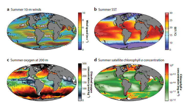
Here on the Oregon Coast, we are perched on the edge of a bountiful upwelling ecosystem. Upwelling is the process by which winds drive a net movement of surface water offshore, which is replaced by cold, nutrient-rich water. When this water full of nutrients meets the sunlight of the photic zone, large phytoplankton blooms occur that sustain high densities of forage species like zooplankton and fish, and yielding important feeding opportunities for predators such as marine mammals. Upwelling ecosystems, like the California Current system in our back yard that features in Duncan Berry’s poem, support over 20% of global fisheries catches despite covering an area less than 5% of the global oceans4–6. These narrow bands of ocean on the eastern boundaries of the major oceans are characterized by strong winds, cool sea surface temperatures, and high primary productivity that ultimately support thriving and productive ecosystems (Fig. 2)7.
Figure 2. Reproduced from Bograd et al. 2023. Maps showing global means in several key properties during the warm season (June through August in the Northern Hemisphere and January through March in the Southern Hemisphere). The locations of the four eastern boundary current upwelling systems (EBUSs) are shown by black outlines in each panel. (a) 10-m wind speed (colors) and vectors. (b) SST. (c) Dissolved oxygen concentrations at 200-m depth. (d) Concentration of ocean chlorophyll a. Abbreviations: BenCS, Benguela Current System; CalCS, California Current System; CanCS, Canary Current System; HumCS, Humboldt Current System; SST, sea surface temperature.
Because of their importance to human societies, eastern boundary current upwelling systems (EBUSs) have been well-studied over time. Now, scientists around the world who have dedicated their careers to understanding and describing the dynamics of upwelling systems are forced to reckon with the looming question of what will happen to these systems under climate change. The state of available information was recently synthesized in a forthcoming paper by Bograd et al. (2023). These authors find that the future of upwelling systems is uncertain, as climate change is anticipated to drive conflicting physical changes in their oceanography. Namely, alongshore winds could increase, which would yield increased upwelling. However, a poleward shift in these upwelling systems will likely lead to long-term changes in the intensity, location, and seasonality of upwelling-favorable winds, with intensification in poleward regions but weakening in equatorward areas. Another projected change is stronger temperature gradients between inshore and offshore areas, and vertically within the water column. What these various opposing forces will mean for primary productivity and species community structure remains to be seen.
While most of my prior research has centered around the importance of productive upwelling systems for supporting marine mammal feeding grounds8–10, my recent focus has shifted closer to home, to the nearshore waters less than 5 km from the coastline. Despite their ecological and economic importance, nearshore habitats remain understudied, particularly in the context of climate change. Through the recently launched EMERALD project, we are investigating spatial and temporal distribution patterns of harbor porpoises and gray whales between San Francisco Bay and the Columbia River in relation to fluctuations in key environmental drivers over the past 30 years. On a scientific level, I am thrilled to have such a rich dataset that enables asking broad questions relating to how changing environmental conditions have impacted these nearshore sentinel species. On a more personal level, I must admit some apprehension of what we will find. The excitement of detecting statistically significant northward shift in harbor porpoise distribution stands at odds with my own grappling with what that means for our planet. The oceans are changing, and sensitive species must move or adapt to persist. What does the future hold for this “wild edge of a continent of ours” that I love, as Duncan Berry describes?
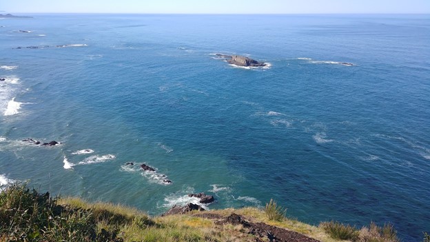
Figure 4. The view from Cape Foulweather, showing the complex mosaic of nearshore habitat features. Photo: D. Barlow.
Evidence exists that the nearshore realm of the Northeast Pacific is actually decoupled from coastal upwelling processes11. Rather, these areas may be a “sweet spot” in the coastal boundary layer where headlands and rocky reefs provide more stable retention areas of productivity, distinct from the strong upwelling currents just slightly further from shore (Fig. 4). As the oceans continue to shift under the impacts of climate change, what will it mean for these critically important nearshore habitats? While they are adjacent to prominent upwelling systems, they are also physically, biologically, and ecologically distinct. Will nearshore habitats act as a refuge alongside a more rapidly changing upwelling environment, or will they be impacted in some different way? Many unanswered questions remain. I am eager to continue seeking out truth in the data, with my drive for scientific inquiry fueled by my underlying connection to this wild edge of a continent that I call home.
Did you enjoy this blog? Want to learn more about marine life, research, and conservation? Subscribe to our blog and get a weekly alert when we make a new post! Just add your name into the subscribe box below!
References:
1. Poloczanska, E. S. et al. Global imprint of climate change on marine life. Nat. Clim. Chang.3, (2013).
2. Lenoir, J. et al. Species better track climate warming in the oceans than on land. Nat. Ecol. Evol.4, 1044–1059 (2020).
3. Hoegh-Guldberg, O. & Bruno, J. F. The impact of climate change on the world’s marine ecosystems. Science (2010). doi:10.1126/science.1189930
4. Mann, K. H. & Lazier, J. R. N. Dynamics of Marine Ecosystems: Biological-physical interactions in the oceans. Blackwell Scientific Publications (1996). doi:10.2307/2960585
5. Ryther, J. Photosynthesis and fish production in the sea. Science (80-. ).166, 72–76 (1969).
6. Cushing, D. H. Plankton production and year-class strength in fish populations: An update of the match/mismatch hypothesis. Adv. Mar. Biol.9, 255–334 (1990).
7. Bograd, S. J. et al. Climate Change Impacts on Eastern Boundary Upwelling Systems. Ann. Rev. Mar. Sci.15, 1–26 (2023).
8. Barlow, D. R., Bernard, K. S., Escobar-Flores, P., Palacios, D. M. & Torres, L. G. Links in the trophic chain: Modeling functional relationships between in situ oceanography, krill, and blue whale distribution under different oceanographic regimes. Mar. Ecol. Prog. Ser.642, 207–225 (2020).
9. Barlow, D. R., Klinck, H., Ponirakis, D., Garvey, C. & Torres, L. G. Temporal and spatial lags between wind, coastal upwelling, and blue whale occurrence. Sci. Rep.11, 1–10 (2021).
10. Derville, S., Barlow, D. R., Hayslip, C. & Torres, L. G. Seasonal, Annual, and Decadal Distribution of Three Rorqual Whale Species Relative to Dynamic Ocean Conditions Off Oregon, USA. Front. Mar. Sci.9, 1–19 (2022).
11. Shanks, A. L. & Shearman, R. K. Paradigm lost? Cross-shelf distributions of intertidal invertebrate larvae are unaffected by upwelling or downwelling. Mar. Ecol. Prog. Ser.385, 189–204 (2009).
To understand the complex dynamics of an ecosystem, we need to examine how physical forcing drives biological response, and how organisms interact with their environment and one another. The largest animal on the planet relies on the wind. Throughout the world, blue whales feed areas where winds bring cold water to the surface and spur productivity—a process known as upwelling. In New Zealand’s South Taranaki Bight region (STB), westerly winds instigate a plume of cold, nutrient-rich waters that support aggregations of krill, and ultimately lead to foraging opportunities for blue whales. This pathway, beginning with wind input and culminating in blue whale occurrence, does not take place instantaneously, however. Along each link in this chain of events, there is some lag time.
Figure 1. A blue whale comes up for air in New Zealand’s South Taranaki Bight. Photo: L. Torres.
Our recent paper published in Scientific Reports examines the lags between wind, upwelling, and blue whale occurrence patterns. While marine ecologists have long acknowledged that lag plays a role in what drives species distribution patterns, lags are rarely measured, tested, and incorporated into studies of marine predators such as whales. Understanding lags has the potential to greatly improve our ability to predict when and where animals will be under variable environmental conditions. In our study, we used timeseries analysis to quantify lag between different metrics (wind speed, sea surface temperature, blue whale vocalizations) at different locations. While our methods are developed and implemented for the STB ecosystem, they are transferable to other upwelling systems to inform, assess, and improve predictions of marine predator distributions by incorporating lag into our understanding of dynamic marine ecosystems.
So, what did we find? It all starts with the wind. Wind instigates upwelling over an area off the northwest coast of the South Island of New Zealand called Kahurangi Shoals. This wind forcing spurs upwelling, leading to the formation of a cold water plume that propagates into the STB region, between the North and South Islands, with a lag of 1-2 weeks. Finally, we measured the density of blue whale vocalizations—sounds known as D calls, which are produced in a social context, and associated with foraging behavior—recorded at a hydrophone downstream along the upwelling plume’s path. D call density increased 3 weeks after increased wind speeds near the upwelling source. Furthermore, we looked at the lag time between wind events and aggregations in blue whale sightings. Blue whale aggregations followed wind events with a mean lag of 2.09 ± 0.43 weeks, which fits within our findings from the timeseries analysis. However, lag time between wind and whales is variable. Sometimes it takes many weeks following a wind event for an aggregation to form, other times mere days. The variability in lag can be explained by the amount of prior wind input in the system. If it has recently been windy, the water column is more likely to already be well-mixed and productive, and so whale aggregations will follow wind events with a shorter lag time than if there has been a long period without wind and the water column is stratified.
Figure 2. Top panel: Map of the study region within the South Taranaki Bight (STB) of New Zealand, with location denoted by the white rectangle on inset map in the upper right panel. All spatial sampling locations for sea surface temperature implemented in our timeseries analyses are denoted by the boxes, with the four focal boxes shown in white that represent the typical path of the upwelling plume originating off Kahurangi shoals and moving north and east into the STB. The purple triangle represents the Farewell Spit weather station where wind measurements were acquired. The location of the focal hydrophone (MARU2) where blue whale D calls were recorded is shown by the green star. (Reproduced from Barlow et al. 2021). Bottom panel: Results of the timeseries cross-correlation analyses, illustrating the lag between some of the metrics and locations examined.
This publication forms the second chapter of my PhD dissertation. However, in reality it is the culmination of a team effort. Just as whale aggregations lag wind events, publications lag years of hard work. The GEMM Lab has been studying New Zealand blue whales since Leigh first hypothesized that the STB was an undocumented foraging ground in 2013. I was fortunate enough to join the research effort in 2016, first as a Masters student and now as a PhD Candidate. I remember standing on the flying bridge of R/V Star Keys in New Zealand in 2017, when early in our field season we saw very few blue whales. Leigh and I were discussing this, with some frustration. Exclamations of “This is cold, upwelled water! Where are the whales?!” were followed by musings of “There must be a lag… It has to take some time for the whales to respond.” In summer 2019, Christina Garvey came to the GEMM Lab as an intern through the NSF Research Experience for Undergraduates program. She did an outstanding job of wrangling remote sensing and blue whale sighting data, and together we took on learning and understanding timeseries analysis to quantify lag. In a meeting with my PhD committee last spring where I presented preliminary results, Holger Klinck chimed in with “These results are interesting, but why haven’t you incorporated the acoustic data? That is a whale timeseries right there and would really add to your analysis”. Dimitri Ponirakis expertly computed the detection area of our hydrophone so we could adequately estimate the density of blue whale calls. Piecing everything together, and with advice and feedback from my PhD committee and many others, we now have a compelling and quantitative understanding of the upwelling dynamics in the STB ecosystem, and have thoroughly described the pathway from wind to whales in the region.
Figure 3. Dawn and Leigh on the flying bridge of R/V Star Keys on a windy day in New Zealand during the 2017 field season. Photo: T. Chandler.
Our findings are exciting, and perhaps even more exciting are the implications. Understanding the typical patterns that follow a wind event and how the upwelling plume propagates enables us to anticipate what will happen one, two, or up to three weeks in the future based on current conditions. These spatial and temporal lags between wind, upwelling, productivity, and blue whale foraging opportunities can be harnessed to generate informed forecasts of blue whale distribution in the region. I am thrilled to see this work in print, and equally thrilled to build on these findings to predict blue whale occurrence patterns.
Reference: Barlow, D.R., Klinck, H., Ponirakis, D., Garvey, C., Torres, L.G. Temporal and spatial lags between wind, coastal upwelling, and blue whale occurrence. Sci Rep 11, 6915 (2021). https://doi.org/10.1038/s41598-021-86403-y
Fall has arrived in the Pacific Northwest. For humans, it means packing away the shorts and sandals, and getting the boots, raincoats and firewood ready. For gray whales, it means gulping down the last meal of zooplankton they will eat for several months and commencing the journey to warmer waters and sunnier skies in Mexico where they will spend the winter fasting, calving, and nursing. While the GEMM Lab may still squeeze in a day or two of field work this week, we are slowly wrapping up the 2020 field season as conditions get rougher and our beloved gray whales gradually depart our waters. This year marked the 6th year of data collection for both of our gray whale projects: the Newport project that investigates the impacts of multiple stressors on gray whale ecology and health, and the Port Orford project that explores fine-scale foraging ecology of gray whales and their zooplankton prey. Since it will be several months before the GEMM Lab heads back out onto the water again, I thought I would summarize our two field seasons, share some highlights, and muse about the drivers of our observations this summer.
Some snapshots of the field team hard at work this summer. Top left: Hunter Warwick operating the drone. Top right: PI Leigh Torres rocking the lab swag to protect against the sun. Bottom left: Lisa Hildebrand waiting for a whale to surface to get photos of it. Bottom right: Alejandro Fernandez Ajo transfers zooplankton from the light trap to sample jars.
Summaries
Our RHIB Ruby zipped around the central and southern Oregon coast on 33 different days. The summer started slow, with several days of field work where we encountered no whales despite surveying our entire study region. Our encounters picked up towards the end of June and by the end of the summer we totaled 107 sightings, encountering 46 unique individuals, 36 of which were resightings of known individuals we have identified in previous years. Our Newport star of the summer was Solé, a female gray whale we have seen every year since 2015, and we also saw many of our other regulars including Casper, Rafael, Spray, Bit, and Heart. None of these whales shone as bright as Solé though. We flew the drone over her 8 times and collected 7 fecal samples (one of which was the biggest whale fecal sample I have ever seen!). In total, we collected 30 fecal samples and flew the drone 88 times. These data will allow us to continue measuring body condition and hormone levels of Pacific Coast Feeding Group (PCFG) gray whales that use the Oregon coast.
Left: Our RHIB Ruby heading out for a day of field work in Port Orford, OR this summer. Right: Solé. Image captured under NOAA/NMFS permit #21678.
Our tandem research kayak Robustus may not be as zippy as Ruby (it is powered by human muscle rather than a powerful outboard engine after all), but it certainly continues to be a trusty vessel for the Port Orford team. The Port Orford research team, named the Theyodelers this year, collected 181 zooplankton samples and conducted 180 GoPro drops during the month of August from Robustus. Despite the many samples collected, the size of our prey samples remained relatively small throughout the whole season compared to previous years. The cliff team surveyed for a total of 117 hours, of which 15 were spent tracking whales with the theodolite and resulted in 40 different tracklines of whale movements. The whale situation in Port Orford was similar to the pattern of whale sightings in Newport, with low whale sightings at the start of the field season. Luckily, by the start of August (which marked the start of data collection for the Theyodelers), the number of whales using the Port Orford area, especially the two study sites, Mill Rocks & Tichenor Cove, had increased. Of the whales that came close enough to shore for us to identify using photo-id, we tracked 5 unique individuals, 3 of which we also saw in Newport this year. The Port Orford star of the summer was Smudge, with his tracklines making up a quarter of all of our tracklines collected. Smudge is also the whale we sighted most often last year in Port Orford.
Top: Theyodelers Mattea Holt Colberg and Liz Kelly sampling atop the kayak Robustus. Bottom: Smudge. Image captured under NOAA/NMFS permit #21678.
Highlights
Many of you may be familiar with the whale Scarlett (formally known as Scarback). Scarlett is a female, at least 24 years old (she was first documented in the PCFG range in 1996), who is well-known (and easily identified) by the large concave injury on her back that is covered in whale lice, or cyamids. No one knows for certain how Scarlett sustained this injury (though there are stories), however what we do know is that it has not prevented this female from reproducing and successfully raising several calves over her lifetime. The GEMM Lab last saw Scarlett with a calf (which we named Brown) in 2016. Since Scarlett is such a famous whale with a unique history, it shouldn’t be a surprise that one of our highlights this summer is the fact that Scarlett showed up with a new calf! In keeping with a “shades of red” theme, Leigh came up with the name Rose for the new calf. In July, the mom-calf pair put on quite a cute performance, with Rose rising up on Scarlett’s back, giving the team a glimpse of its face. The Scarlett-Rose highlight doesn’t end there though. Just last week, we had a very brief encounter in choppy, swelly waters with a small whale. The whale surfaced just twice allowing us to capture photo-id images, and as we were looking around to see where it would come up a third time, it suddenly breached approximately 20 m from the boat. Lo-and-behold, after comparing our photos of the whale to our catalogue, we realized that this elusive, breaching whale was Rose! I am excited to see whether Rose will return to the Oregon coast next summer and become a PCFG regular just like her mom.
Top: Scarlett, easily identified by the large concave injury on her back covered in cyamids. Bottom: Scarlett with her new calf Rose riding her back, giving us a glimpse of its face. Images captures under NOAA/NMFS permit #21678.
The highlight of the field season in Port Orford is the trial, failures and small successes of a new element to the project. There is still a lot that we do not know and understand about PCFG gray whales. One such thing is the way in which gray whales maneuver their large bodies in shallow rocky habitats, often riddled with kelp, and how exactly they capture their zooplankton prey in these environments. Using drones has certainly helped bring some light into this darkness and has led to the documentation of many novel foraging behaviors (Torres et al. 2018). However, the view from above is unable to provide the fine-scale interactions between whales, kelp, reefs, and zooplankton. Instead, we must somehow find a way to watch the whales underwater. Enter CamDo. CamDo is a technology company that designs specialty products to allow for GoPro cameras to be used for time-lapsed recordings over long periods of time in harsh environmental conditions. One of their products is a housing specifically designed for long-term filming underwater – exactly what we need! The journey was not as easy as simply purchasing the housing. We also needed to build a lander for the housing to sit on (thankfully our very own Todd Chandler designed and built something for us), and coordinate with divers and a vessel to deploy and retrieve the set-up, as well as undertake weekly battery and SD cards swaps (thankfully Dave Lacey of South Coast Tours and a very generous group of divers* donated their time and resources to make this happen). We unfortunately had some technological difficulties and bad visibility for the first 4 weeks (precisely why this CamDo effort was a pilot season this year), however we had some small success in the last 2 weeks of deployment that give us hope for the future. The camera recorded a lot of things: thick layers of mysids, countless rockfish and lingcod, several swimming and foraging murres, a handful of harbor seals, and two encounters of the species we were hoping to film – gray whales! While the footage is not the ‘money shot’ we are hoping to film (aka, a headstanding gray whale eating zooplankton right in front of the camera), the fact that we captured gray whales in the first place has showed us that this set-up is a promising investment of time, money and effort that will hopefully deliver next year.
Top left: CamDo atop its lander designed and built by Todd Chandler. Top right: Divers getting ready to get into the water for a battery and SD card swap. Bottom: Dave Lacey and two of our divers with the Black Pearl, South Coast Tour’s boat.
Musings
You may have picked up on the fact that we had slow starts to our field seasons in both Newport and Port Orford. Furthermore, while the number of whale sightings did increase in both locations throughout the field seasons, the number of sightings and whales per day were lower than they have been in previous years. For example, in 2018, we identified 15 different individuals in the month of August in Port Orford (compared to just 5 this year). In 2019, 63 unique whales were seen in Newport (compared to 46 this year). Interestingly, we had a greater diversity of encountered individuals at the start and end of the season in Newport, with a relatively small number of different individuals in July and August. While I cannot provide a definitive reason (or reasons) as to why patterns were observed (we will need to analyze several years of our data to try and understand why), I have some hypotheses I wish to share with you.
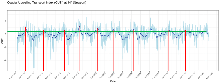
As I mentioned in a previous blog, this summer the coastal upwelling along the Oregon coast was delayed (Figure 1). Typically, peak upwelling occurs during the month of June or shortly thereafter, bringing nutrient-rich, deep waters to the surface and, when mixed with sunlight, a lot of productivity. This productivity sets off a chain of reactions — the input of nutrients leads to increased phytoplankton production, which in turn leads to increased zooplankton production, resulting in growth and development of larger organisms that consume zooplankton, such as rockfish and gray whales. If the timing of upwelling is delayed, then so too is this chain of reactions. As you can see from Figure 1, the red lines show that the peak upwelling this year occurred far later in the summer than any year in the last 10 years, with the exception of 2012. Gray whales may have cued into this delay and therefore also delayed their arrival to the PCFG feeding grounds, hence causing us to have low sighting rates at the start of our season. However, this is mostly speculative as we still do not understand the functional mechanisms by which cetaceans, such as gray whales, detect prey across different scales, and to what extent oceanographic conditions like upwelling may play a role in prey availability (Torres 2017).
Figure 1. 10 year time series of the Coastal Upwelling Transport Index (CUTI). CUTI represents the amount of upwelling (positive numbers) or downwelling (negative numbers). The light-colored lines representthe CUTI at that point in time while the dark, bold line represents the long-term average.The vertical red lines represent the point of peak upwelling in that summer and the horizontal green line shows the peak level of upwelling in 2020 relative to all previous years.
Furthermore, the green line in Figure 1shows that even after peak upwelling was reached this year, upwelling conditions were lower than all the other peaks in the previous 10 years. We know that weak upwelling is correlated to poor body condition of PCFG gray whales in subsequent years (Soledade Lemos et al. 2020). Upon arriving to the Oregon coast feeding grounds, gray whales may have noticed that it was shaping up to be a poor prey year (we certainly noticed it in Port Orford in the emptiness of our zooplankton net). Faced with this low resource availability, individuals had to make important decisions – risk staying in a currently prey-poor environment or continue the journey onward, searching for better prey conditions elsewhere. This conundrum is known as the marginal value theorem, whereby an individual must decide whether it should abandon the patch it is currently foraging on and move on to search for a new patch without knowing how far away the next patch may be or its value relative to the current patch (Charnov 1976). If we think of the Oregon coast as the ‘current patch’, then we can see how the marginal value theorem translates to the situation gray whales may have found themselves in at the start of the summer.
Yet, an individual gray whale does not make these decisions in a vacuum. Instead, all gray whales in the same area are faced with the same conundrum. Seminal work by Pianka (1974) showed that when resources, such as food, are abundant, then competition between predators is low because there is enough food to go around. However, when resources dwindle, competition increases and the niches of predators begin to overlap more and more. With Charnov and Pianka’s theories in mind, we can see two groups of gray whales emerge from our 2020 field work observations: those that stayed in the ‘current patch’ (Oregon) and those that decided to seek out a new patch in hopes that it would be a better one. Solé certainly belongs in the first group. We saw her consistently throughout the whole summer. In fact, she was oftentimes so predictable that we would find her foraging on the same reef complex every time we went out to survey. Smudge may also belong in this group, however it is hard to say definitively since we only survey in Port Orford in late July and August. In contrast, I would place whales such as Spray and Heart in the second group since we saw them early in the summer and then not again until mid-to-late September. Where did they go in the interim? Did they go somewhere else in the PCFG range? Or did they venture all the way up to Alaska to the primary Eastern North Pacific (ENP) gray whale feeding grounds? Did their choice to search for food elsewhere pay off?
As I said earlier, these are all just musings for now, but the GEMM Lab is already hard at work trying to answer these questions. Stay tuned to see what we find!
* Thanks to all the divers who assisted with the pilot CamDo season: Aaron Galloway, Ross Whippo, Svetlana Maslakova, Taylor Eaton, Cori Kane, Austin Williams, Justin Smith
References
Charnov, E.L. 1976. Optimal Foraging, the Marginal Value Theorem. Theoretical Population Biology 9(2):129-136.
Pianka, E.R. 1974. Niche Overlap and Diffuse Competition. PNAS 71(5):2141-2145.
Soledade Lemos, L., Burnett, J.D., Chandler, T.E., Sumich, J.L., and L.G. Torres. 2020. Intra- and inter-annual variation in gray whale body condition on a foraging ground. Ecosphere 11(4):e03094.
Torres, L.G. 2017. A sense of scale: Foraging cetaceans’ use of scale-dependent multimodal sensory systems. Marine Mammal Science 33(4):1170-1193.
Torres, L.G., Nieukirk, S.L., Lemos, L., and T.E. Chandler. 2018. Drone Up! Quantifying Whale Behavior From a New Perspective Improves Observational Capacity. Frontiers in Marine Science: https://doi.org/10.3389/fmars.2018.00319.
The focus of my PhD research is on the ecology and distribution of blue whales in New Zealand. However, it has been a long time since I’ve seen a blue whale, and much of my time recently has been spent thinking about wind. What does wind matter to a blue whale? It actually matters a whole lot, because the wind drives an important biological process in many coastal oceans called upwelling. Wind blowing along shore, paired with the rotation of the earth, leads to a net movement of surface waters offshore (Fig. 1). As the surface water is pushed away, it is replaced by cold, nutrient-rich water from much deeper. When those nutrients become exposed to sunlight, they provide sustenance for the little planktonic lifeforms in the ocean, which in turn provide food for much larger predators including marine mammals such as blue whales. This “wind-to-whales” trophic pathway was coined by Croll et al. (2005), who demonstrated that off the West Coast of the United States, aggregations of whales could be expected downstream of upwelling centers, in concert with high productivity and abundant krill prey.
Figure 1. Graphic of the upwelling process, illustrating that when the wind blows along shore, surface waters are replaced by deeper water that is cold and nutrient rich. Source: NOAA
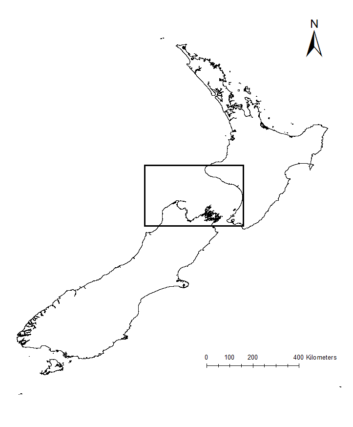
Figure 2. Map of New Zealand, with the South Taranaki Bight region (STB) denoted by the black box.
Much of what is understood today about upwelling comes from decades of research on the California Current ecosystem off the West Coast of the United States. Yet, the focus of my research is on an upwelling system on the other side of the world, in the South Taranaki Bight region (STB) of New Zealand (Fig. 2). In the case of the STB, westerly winds over Kahurangi Shoals lead to decreased sea level nearshore, forcing cold, nutrient rich waters to rise to the surface. The wind, along with the persistence of the Westland Current, then pushes a cold and productive plume of upwelled waters around Cape Farewell and into the STB (Fig. 3; Shirtcliffe et al. 1990).
Figure 3. Satellite image of the cold water plume in the South Taranaki Bight, indicative of upwelling. The origin of the upwelling at Kahurangi Shoals, Cape Farewell, and the typical path of the upwelling plume are denoted.
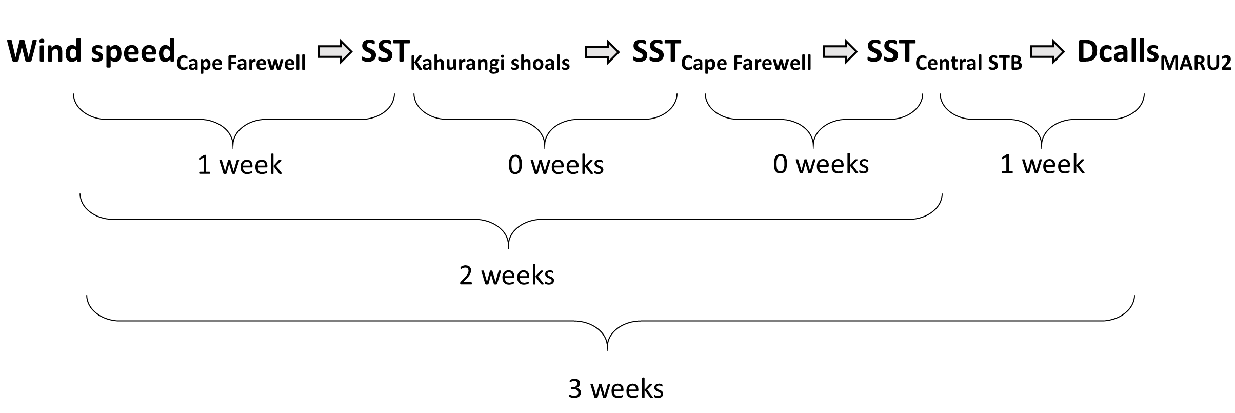
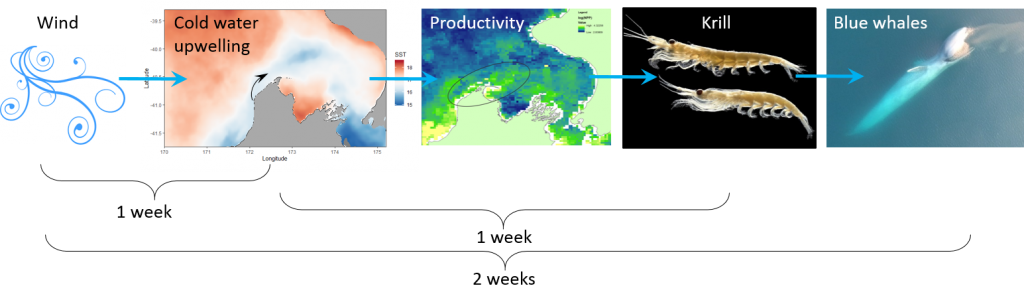
Through research conducted by the GEMM Lab over the years, we have demonstrated that blue whales utilize the STB region for foraging (Torres 2013, Barlow et al. 2018). Recent research on the oceanography of the STB region has further illuminated the mechanisms of this upwelling system, including the path and persistence of the upwelling plume in the STB across years and seasons (Chiswell et al. 2017, Stevens et al. 2019). However, the wind-to-whales pathway has not yet been described for this part of the world, and that is where the next section of my PhD research comes in. The whole system does not respond instantaneously to wind; the pathway from wind to whales takes time. But how much time is required for each step? How long after a strong wind event can we expect aggregations of feeding blue whales? These are some of the questions I am trying to tackle. For example, we hypothesize that some of the mechanisms and their respective lag times can be sketched out as follows:
Figure 4. The wind-to-whales trophic pathway, and hypothesized lags between steps.
All of these questions involve integrating oceanography, satellite imagery, wind data, and lag times, leading me to delve into many different analytical approaches including time series analysis and predictive modeling. If we are able to understand the lag times along this series of events leading to blue whale feeding opportunities, then we may be able to forecast blue whale occurrence in the STB based on the current wind and upwelling conditions. Forecasting with some amount of lead time could be a very powerful management tool, allowing for protection measures that are dynamic in space and time and therefore more effective in conserving this blue whale population and balancing human impacts.
Figure 5. A blue whale lunges on a patch of krill. The end of the wind-to-whales pathway. Drone piloted by Todd Chandler.
References:
Barlow DR, Torres LG,
Hodge KB, Steel D, Baker CS, Chandler TE, Bott N, Constantine R, Double MC,
Gill P, Glasgow D, Hamner RM, Lilley C, Ogle M, Olson PA, Peters C, Stockin KA,
Tessaglia-hymes CT, Klinck H (2018) Documentation of a New Zealand blue whale
population based on multiple lines of evidence. Endanger Species Res 36:27–40.
Chiswell SM, Zeldis JR,
Hadfield MG, Pinkerton MH (2017) Wind-driven upwelling and surface chlorophyll
blooms in Greater Cook Strait. New Zeal J Mar Freshw Res.
Croll DA, Marinovic B,
Benson S, Chavez FP, Black N, Ternullo R, Tershy BR (2005) From wind to whales:
Trophic links in a coastal upwelling system. Mar Ecol Prog Ser 289:117–130.
Shirtcliffe TGL, Moore
MI, Cole AG, Viner AB, Baldwin R, Chapman B (1990) Dynamics of the Cape
Farewell upwelling plume, New Zealand. New Zeal J Mar Freshw Res 24:555–568.
Stevens CL, O’Callaghan
JM, Chiswell SM, Hadfield MG (2019) Physical oceanography of New
Zealand/Aotearoa shelf seas–a review. New Zeal J Mar Freshw Res.
Torres LG (2013)
Evidence for an unrecognised blue whale foraging ground in New Zealand. New
Zeal J Mar Freshw Res 47:235–248.