Return of The Kelp? Cascading Conditions in Port Orford

Owen Fewell, GEMM Lab TOPAZ/JASPER Intern, OSU Fisheries, Wildlife, and Conservation Sciences Undergraduate

Hello! I’m Owen Fewell, the OSU undergraduate intern on the TOPAZ/JASPER project. I’ll be going into my senior year at Oregon State University, majoring in Fisheries, Wildlife, and Conservation Sciences. I am originally from Marin County, about 40 minutes north of San Francisco, CA. My interest in the ocean stems from fond memories I share with my family, where almost any free time we had would be spent on the coast hiking, kayaking, or enjoying the beach. Truthfully, I never loved ocean kayaking as a kid because of how tiring it was, but things have definitely changed now, as that experience allowed me to be a part of this amazing project.

**Fig 1**: Picture of me during the first week of training in Port Orford. The team conducted a scavenger hunt-type activity to learn how to use a GPS, and we now apply this newfound knowledge to locate our sampling sites on the water.

As I am writing this, I find it hard to believe our team has already been here for three weeks. The TOPAZ/JASPER internship is my first exposure to real data collection, and my time here has been great so far. The work can be tedious at times, so it has been crucial to stay calm and remember all of the necessary steps in the process. Our days are jam packed with fieldwork, either navigating toward our 12 stations on the kayak to collect data, scanning for gray whales on the horizon from the bluff, or identifying the many different types of zooplankton we collect. Each day presents new and unique challenges that our team couldn’t have expected – from unpredictable ocean conditions to sporadic beeping signals on the theodolite, we have to be prepared for it all. Luckily, we have our fearless leader Celest, who is always able to adapt and show us how to find solutions under pressure. So far this season the only problem that we can’t seem to solve is the lack of whales! There have been a couple reported sightings of whales coming through while we’ve been here, but only later in the evening once we packed everything up. By reading different publications built off data collected from this project in previous years, and hearing from Port Orford locals and prior interns, we’ve learned that this absence of whales isn’t completely random, but the result of a changing ecosystem.

**Fig 2.** Fellow TOPAZ/JASPER intern Adrian Ruiz (right) and I (left) getting ready to embark on one of our first days of kayak training, where we are hoping to get more comfortable navigating to our different stations.

An ecological interest of mine has always been learning more about various forms of tropic cascades, and how the presence or absence of one species can have profound effects on an entire ecosystem. Part of our internship has involved reading literature relevant to our study system here in Port Orford, with our most recent read being “Exploring indirect effects of a classic trophic cascade between urchins and kelp on zooplankton and whales” by Hildebrand et. al. in 2024. In recent years, purple sea urchins, a natural predator for bull kelp, have proliferated in population numbers due to the loss of the urchin’s natural predator, the sunflower sea star. From 2013-2016, a well documented marine heat wave and the development of sea star wasting disease led to the 100% decline of the sunflower sea star population off the coast of Port Orford (Hildebrand et al. 2024). A trophic cascade was observed using the methods that our team currently use during this internship. Specifically, one method involves lowering an oceanographic sensor, the RBR, with a Go-Pro camera attached to simultaneously record differences in temperature and salinity at different depths, alongside video. Additionally, at each site we conduct a small net tow in order to collect zooplankton samples. In Hildebrand et. al. (2024), these methods were performed over 8 years (2016-2023) to connect the purple sea urchin population increase to gray whale foraging habits. As the years progressed, the increase in purple sea urchin correlated with the loss of bull kelp. Since bull kelp provide protection and nutrients to zooplankton, this loss of kelp correlated with a decrease in zooplankton abundance. With less prey available, the Pacific Coast Feeding Group (PCFG) of gray whales were observed less within our study system.

**Fig 3.** Graphic from Hildebrand et. al. (2024) showing Go-Pro footage of bull kelp forests in Port Orford before the tropic cascade (A and B) vs after (C and D) at the same sampling sites

**Fig 4.** Two still images from Go-Pro footage that we’ve taken this year, two years after Hildebrand et. Al (2024) was published. Image A is from station MR19 (Mill Rocks), and image B is from station TC4 (Tichenor’s Cove), the same stations as images from Fig 3.

With our team out on the water everyday collecting zooplankton samples and later reviewing our GoPro videos, I find we observe this dynamic in real time. From recounts of Port Orford locals, Mill Rocks, which is one of our sampling sites, has historically been extremely productive. There were once masses of bull kelp and zooplankton, resulting in somewhat of a hotspot for gray whales. As this is my first time in Port Orford, I only have a vague idea of what conditions used to look like, but there appears to be significantly less kelp than there once was. Specifically, at one of our Mill Rocks sites, former interns have relied on grabbing on to kelp to help keep the kayak steady in the rough water. Unfortunately, throughout our field season we haven’t been able to enjoy this luxury, and instead have had to either brave the rough waters, or abandon the site altogether. However, efforts to reduce these urchin predation pressures and restore kelp habitats are exhibited through a different research group, the Oregon Kelp Alliance (ORKA), where they are actively removing urchins from select areas, and surveying to track the progress of bull kelp regrowth (https://www.oregonkelp.com/the-oregon-kelp-alliance/).

Although the team hasn’t observed as much kelp at our two study sites, we have observed large patches of kelp in different areas, specifically the open water between Mill Rocks and Tichenor’s Cove. I find these new areas with kelp to be interesting, as I am curious to know whether our PCFG gray whales will end up changing their preferred foraging sites according to these new patches and if our project will have to adapt with this changing environment.

A fundamental part of this internship has been learning how to become adaptable, and this is particularly true for the navigator on the kayak. For me, this has been the most difficult yet rewarding job. The navigator that sits at the bow of the tandem kayak must locate each of the 12 stations. Once there, they are responsible for maintaining the kayak within 5 meters of a given station while their partner engages in data collection (e.g., secchi disk, net tow, GoPro drop). Being navigator is physically demanding and can be extremely tedious, as one wrong paddle can lead to being pushed far off the station. Because of the challenge, it makes getting to all 12 stations that much more rewarding.

**Fig 5.** (*left pic*.) This was taken during our first week of kayak training, where I am navigator at the bow, and my fellow intern on the TOPAZ/JASPER project Gavin Vierra is sampler at the stern.
(*right pic.*) Photo of me (left), Adrian (middle left), Celest (middle right), and Gavin V. (right) on our first day off visiting the natural bridges in Brookings.

Being immersed in this coastal ecosystem for the last three weeks, alongside reading research papers, and talking to fellow interns staying at our field station has taught me so much about how a tropic cascade has changed how species are interacting here in Port Orford, and why we might not be observing any gray whales this season. I have also learned about myself, how to stay calm in the field when things aren’t going as planned. I’m really looking forward to the next three weeks, as I have been loving spending time with the team either out on the field or watching movies after our long days (some of my favorites have been Transformers, or Twilight –surprisingly good.) We’re all hoping to see some whales, and put our cliff-side theodolite tracking skills to the test. Regardless, we know the data we’re collecting is still informative to this long-term (12 years and counting!) project and will help to understand why this year has been so different to previous years. All we can do is keep thinking positive thoughts, as according to our team leader Celest, the whales can tell if we aren’t!

References:

Hildebrand, L., Derville, S., Hildebrand, I., & Torres, L. G. (2024). Exploring indirect effects of a classic trophic cascade between urchins and kelp on zooplankton and whales. Scientific Reports, 14(1), 9815. https://doi.org/10.1038/s41598-024-59964-x

Scanning for whales with Sharp Eyes and Smooth Riffs: Meet Team Quick-with-it

Celest Sorrentino, GEMM Lab MSc Student, OSU Department of Fisheries, Wildlife and Conservation Sciences, Geospatial Ecology of Marine Megafauna Lab

July has rolled around just as quickly as the coastal winds sweep across the south coast of Oregon, bringing in a new team for the 2026 TOPAZ/JASPER field season, the projects’ 12^th year in the running. This season also marks my third summer as part of the long-standing TOPAZ/JASPER legacy: first learning the ropes alongside Team Protein and master’s student Allison Dawn in 2024, then growing into my role as the on-site lead for Team Dabwich in 2025 with both Leigh and Lisa’s invaluable guidance from Newport, and now returning once again to guide the 2026 team.

With each season, I have gained a deeper appreciation for the collaboration and genuine passion required to sustain a long-term project like ours. I am especially grateful for the foundation created by previous master’s students Florence Sullivan, Lisa Hildebrand, and Allison Dawn, and for Leigh’s unwavering dedication and effort for TOPAZ/JASPER to continue year after year. Now a week and a half into the field season, the team has completed their first 10-day stretch of training, and morale remains just as high as it was on day one. Each year unites an entirely new and exciting mix of undergraduate and high school interns, and the 2026 team is no exception.

Adrian Ruiz got a head start by joining the GEMM lab in June as our NSF REU intern for this summer. Originally from Santa Rosa, Adrian just completed his second year at CSU Monterey Bay studying Marine Science. Using a microscope to identify tiny bits in the water is no new feat, since at CSUMB he interned along Dr. Matt Scott Savoca and Chad King identifying microplastics from water samples taken in the Monterey Bay area, as part of a larger project investigating the potential health risk for marine mammals. As the oldest brother of three, Adrian naturally acts as a gentle instructive team member for the younger interns.

(left) Adrian reviewing drone footage of pygmy blue whale mother-calf pairs using BORIS for his REU project. (middle) Celest and Adrian out on the kayak in PO. (right) Adrian and fellow TOPAZ/JASPER HS intern Gavin C working together as cliff team.

Gavin Vierra is one of our high school interns residing in Lakeside, OR. Gavin was one of our first applicants for the TOPAZ/JASPER project this year, where his curious spirit shined through. Having spent most of his life fishing and kayaking, spending a few hours on the water is nothing new. However, Gavin is truly in his element when cooking, as his love for making others feel at home manifests in delicious pasta meals for post-fieldwork dinner, such as chicken alfredo and three-cheese penne.

(left) Gavin V with his grandmother and nephew in California. (middle) Gavin V. whipping up some French Toast for the team. (right) Gavin V and Adrian learning how to ocean kayak in sync during our kayak training with Southcoast Tours.

Owen Fewell is an upcoming senior at OSU studying Fisheries and Wildlife. Originally from Marin County, CA, his earliest memories begin in the outdoors, ocean kayaking along the dynamic coastline of Point Reyes with his parents. Also, an older brother like Adrian, Owen’s personality as a natural jester helps keep morale high even after spending 5 hours navigating to our stations.

(left) Throwback picture of Owen ocean kayaking with his parents in Point Reyes. (middle) Celest, Owen, and Gavin V out on the kayak in Tichenor Cove after completing all of Mill Rocks stations. (right) Owen and Adrian practicing some stability at Natural Bridges.

Gavin Cada is our second high school intern from Brookings-Harbor High School. Having moved to the south coast from Las Vegas, NV, just this past year, the coastal system is an entirely new world. In Nevada, Gavin became fascinated with wildlife, taking photographs of birds and reptiles. Now, as part of the TOPAZ/JASPER project, he spends each day on the cliff, eager for a gray whale visitor to finally put his photography skills to the test.

(left) Gavin C. learning how to use a microscope and processing a zooplankton sample. (right) Gavin C. creating a “start fix” to start out cliff team’s observation effort.

Although whales haven’t been observed quite yet, morale remains high both out on the cliff and on the water. Reports of whale sightings prior to the team’s arrival, and the hope of witnessing a gray whale surface alongside while on the kayak, continue to inspire each morning’s 6:30 AM wake up. Through challenging waves and long hours scanning the horizon, this team has found the best way to stay sharp is through riffing off one another and testing each other with some of the best riddles Reddit has to offer. The team has also enjoyed gearing up for the next day by watching the Transformers movies, and carrying that same action-movie intensity onto the water by dramatically narrating our paddles: “In a world where light meets darkness, two men. One kayak. One dream. Twelve stations. Countless zooplankton. Missing whales. Their mission: brave the insurmountable waves and descend into the unforgiving depths to retrieve the samples that could save the planet. This summer…”

(top) Owen and Gavin paddling out to Mill Rocks together.

(bottom-left): Gavin V. introduced the team to a super niche Coos Bay favorite: Vinny’s Smokin’ Burgers! (bottom-right) A few of our team members (Gavin V., Adrian, Owen, and Celest) visiting Natural Bridges to celebrate completing their first 10-day stretch of training.

With their quick comebacks and eagerness to get out on the water, even if actually launching quickly still needs some work, it only seemed fitting to name this year’s crew: Team Quick-with-it.

With plenty of running jokes and action-movie-level determination, Team Quick-With-It is ready to take on the 12th TOPAZ/JASPER field season. Now, we await the whales!

Returning to the ocean with open ears

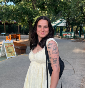
Mariam Alsaid, GEMM Lab Research Technician

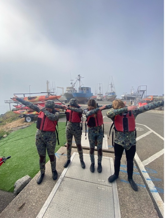
It’s been three years since I last wrote a blog post for the GEMM Lab. At the time, I was wrapping up a wonderful summer filled with science, sun, and new friends and was eager to share all that I had learned and accomplished during my 10 weeks working on the Oregon coast as part of Hatfield Marine Science Center’s Research Experience for Undergraduates (REU). My love and concern for our oceans and its animals has always been the driving force of my academic pursuits. I am so thankful to this REU – funded by the US National Science Foundation – for introducing me to marine science research as a career path.

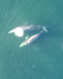
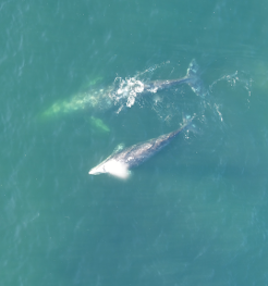
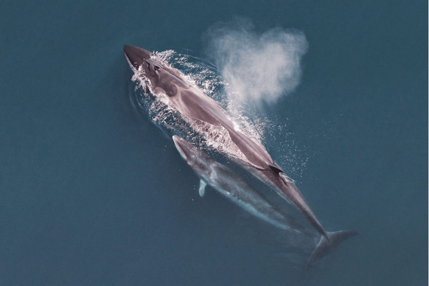
Alongside the mentorship of Drs. Dawn Barlow and Leigh Torres, I investigated the occurrence of sei whales, an endangered species of baleen whale, offshore of Oregon. The sei whale’s global population is believed to have dropped by 80% due to whaling in the 19th and 20th centuries and little is known about their contemporary population status, especially in the Northeast Pacific (Horwood, 2018; Nieukirk et al., 2020). Sei whales have occasionally been observed by the GEMM Lab on research cruises and we were curious about when and how often they were in our neck of the woods. Despite being massive animals (the 3rd largest rorqual in the world!), these animals are challenging to study due to their low population densities and visual similarities to fin whales (Horwood, 2018, Reeves et al., 1998). Luckily, sei whales produce characteristic vocalizations that can help distinguish them from other baleen whales that call at similar frequency bandwidths (e.g. blue, fin, and humpback whales).

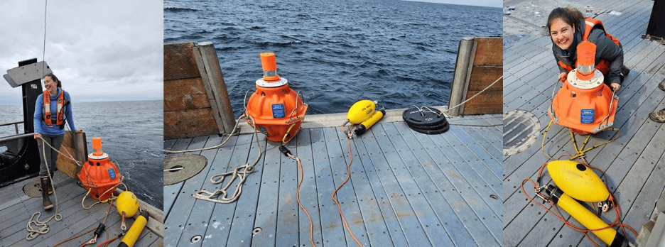
*Figure 1. Sei whale mom and calf (NOAA fisheries)*

This is where bioacoustics – the study of sounds produced by living organisms – comes in. We are able to study this elusive species by deploying hydrophones (underwater microphones) offshore of Oregon and reviewing recorded data in search of sei whale calls. (See this blog post if you’re curious about our methods and findings!).

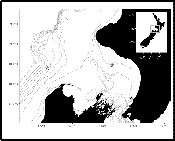
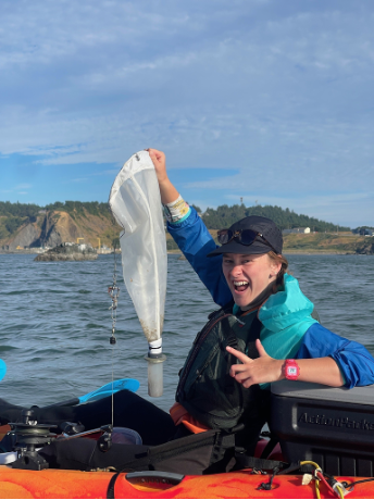
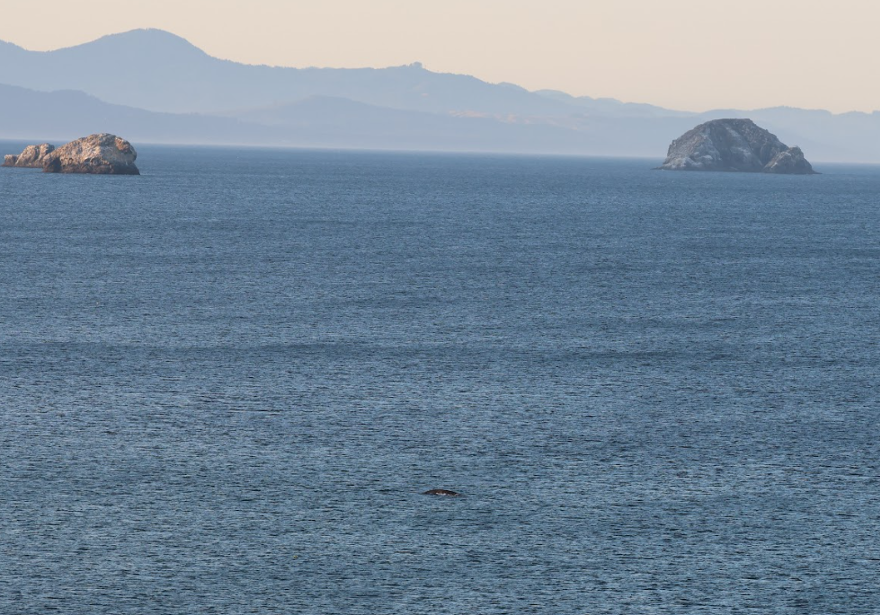
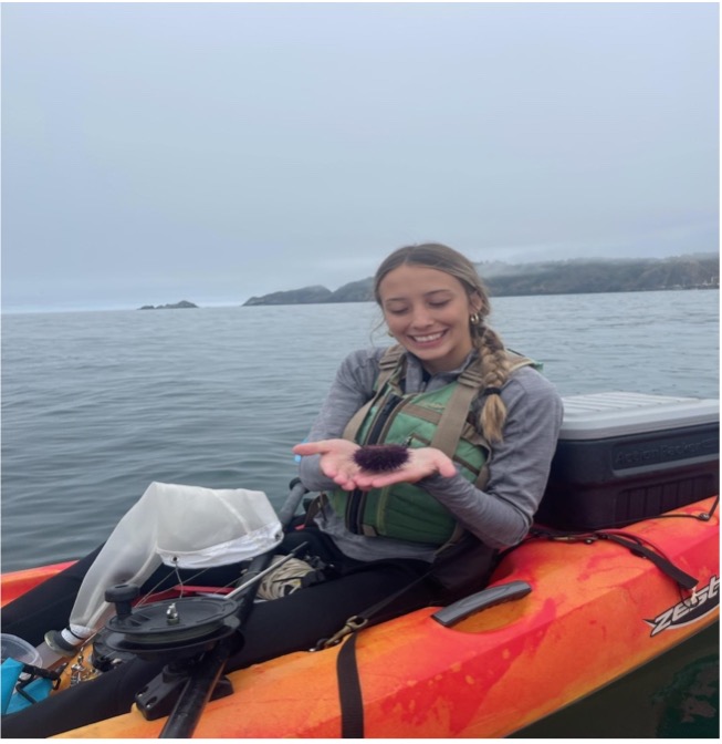
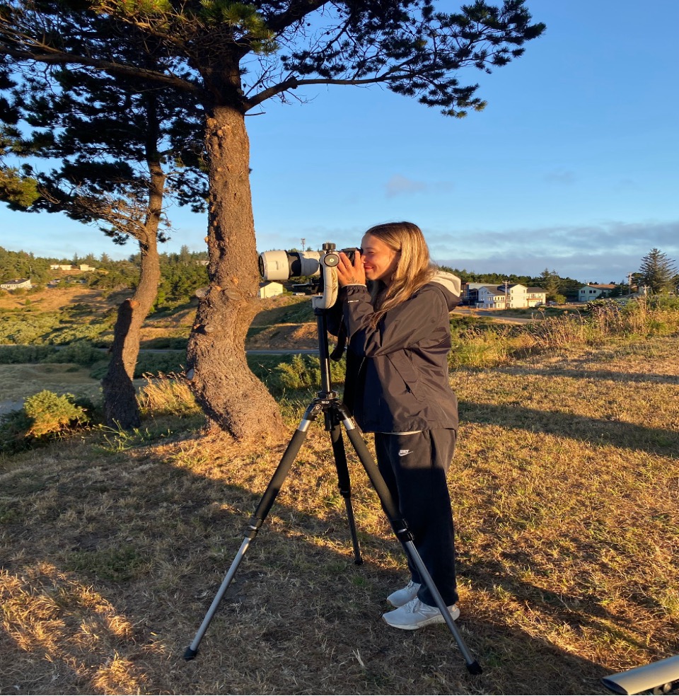
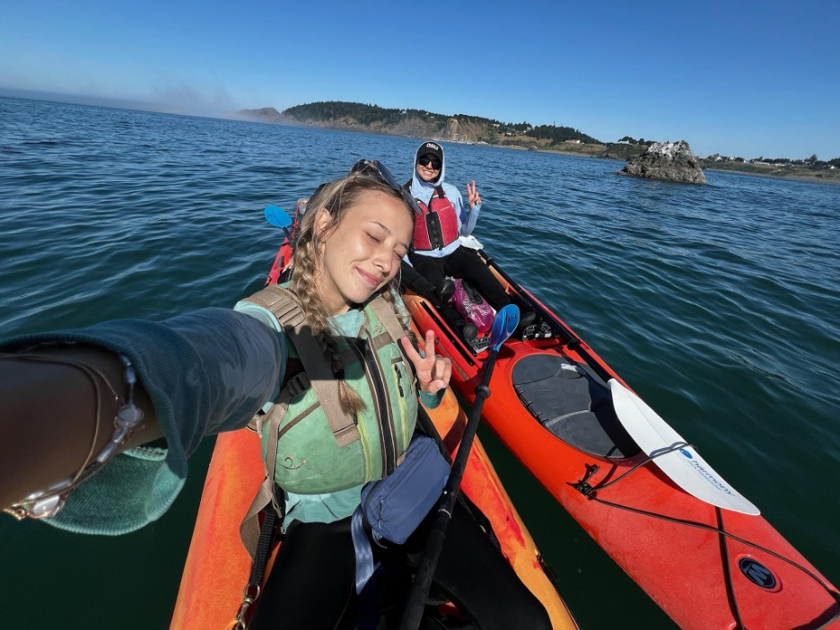
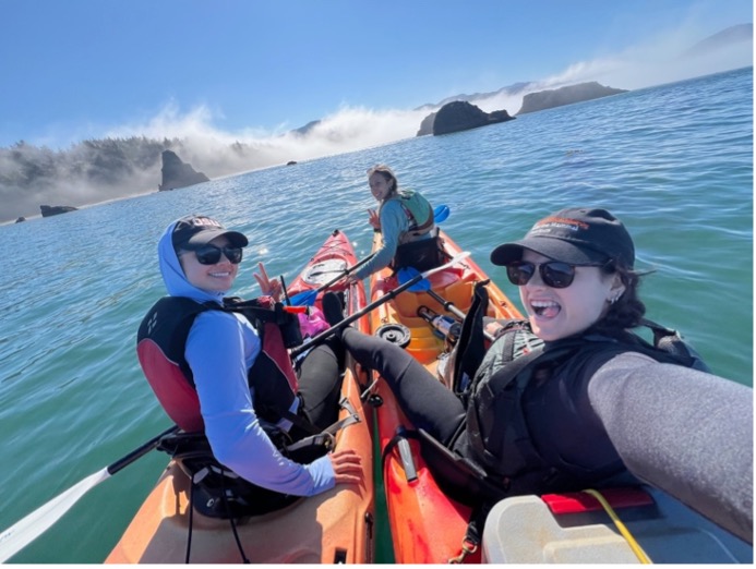
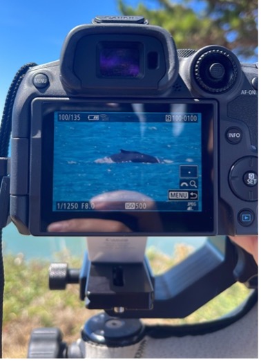
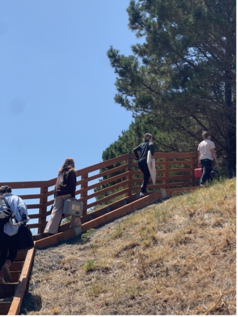
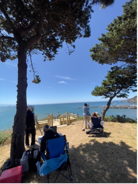
Since 2021, the GEMM Lab and the K. Lisa Yang Center for Conservation Bioacoustics at Cornell University have collaborated to deploy three hydrophones for continuous acoustic recording along the Newport Hydrographic Line as part of the Holistic Assessment of Living marine resources off Oregon (HALO) project. These hydrophones are bottom mounted to the seafloor and are deployed 20, 45, and 65 nautical miles offshore of Newport, OR. HALO cruises are scheduled to refurbish and redeploy these instruments every six months or so. These cruises are also an opportunity to conduct visual surveys of cetaceans and seabirds in between deployments.

*Figure 2. Hydrophone deployments on one of our HALO cruises. Dr. Dawn Barlow pictured on the left and Marrissa Garcia pictured on the right.*

I immediately fell in love with bioacoustics and was enraptured by the diversity of clicks, pulses, and moans made by marine animals that flood our oceans. Hydrophones are able to record sounds in locations and frequency ranges that we would never naturally get to experience. Baleen whales are especially fascinating because they tend to produce infrasonic calls (i.e., <20 Hz) to communicate over large distances. These calls occur at frequencies below our hearing range and are only audible when sped up. Listening to these recordings feels like a window into a secret world that few have ventured.

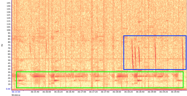
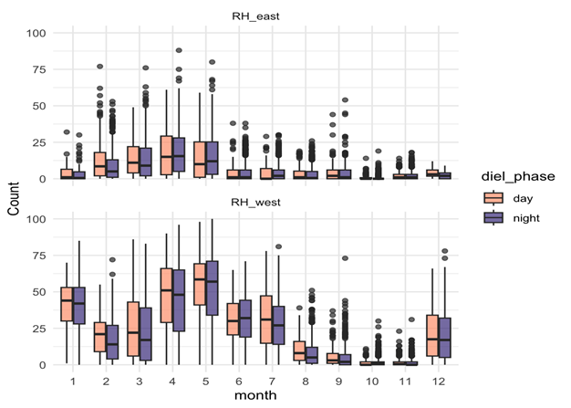
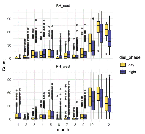
Figure 3. Period of high vocal activity from blue whales (A, B, and D calls), fin whales (20 Hz pulses) , and rockfish (pulses). Audio was sped up by 5x.

After completing my undergraduate degree, I participated in a bioacoustics research fellowship hosted by the US Forest Service and Oak Ridge Institute for Science and Education. During this time, I explored the world of terrestrial acoustics by leading a research project on American pika occupancy in the Oregon and Washington Cascades. Forest soundscapes have a different beauty to them. While periods of quiet are rare in the ocean, this is even scarcer on the surface. Bird songs, insect buzzing, human chatter, rainfall, and highway noise constantly fill our soundscapes, sometimes simultaneously. This experience processing terrestrial sound gave me a newfound appreciation for the world around me and the sounds I’ve become so accustomed to hearing. Nevertheless, I found myself yearning for the ocean and its secrets.

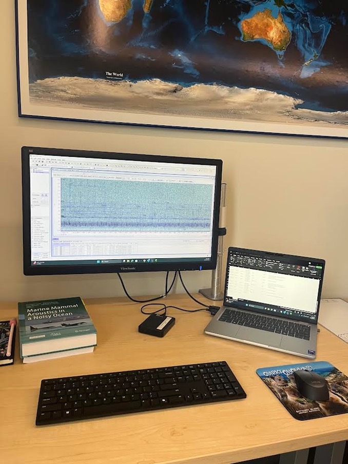
*Figure 3. The typical work setup of an acoustic analyst (headphones, extra hard drives, and coffee missing from photo)*

I was invited back to the Marine Mammal Institute last fall as the GEMM Lab’s baleen whale acoustic analyst to continue working on the HALO project. I dove back into the data collected from our hydrophones, this time targeting blue, fin, and humpback whale calls in addition to sei whales. My efforts were also broadened to all five years of recording data instead of just one. Because manually reviewing large amounts of acoustic data can be cumbersome, I trained artificial intelligence classifiers using the BirdNET convolutional neural network to make acoustic data processing more efficient. After much iterative trial and error, I was able to develop a set of four classifiers, each specialized to detect one of our four target species. The first classifier was trained to target blue whale A, B, and D calls; the second targets fin whale 20 Hz and 40 Hz pulses; the third targets sei whale downsweeps; and the fourth targets humpback song and single non-song grunts. Once I evaluated that the classifiers were performing with high precision and recall rates, I used them to predict when calls occurred in the five years of recording data. I am currently in the process of validating the hundreds of thousands of predictions to generate detection histories of these species of baleen whales in this region. This information will be incorporated with various oceanographic datasets to get a better understanding of baleen whale distribution patterns and habitat preferences in the Northeast Pacific.

I will be wrapping up my contract with the Marine Mammal Institute next month and I am endlessly grateful to the GEMM Lab for shaping me into the marine mammalogist I am today. I will look back on my time here fondly as I begin this next chapter of my life as a PhD student at the University of Washington’s School of Oceanography this fall. I am excited to share that I will continue to use acoustics to study baleen whales in the Northeast Pacific during my PhD! Although I dread the thought of having to say goodbye to Oregon and the Hatfield community, I thankfully won’t have to say goodbye to the whales.

Works cited

Horwood, J. (2018). Sei Whale – Balaenoptera borealis. Encyclopedia of Marine Mammals

(Third Edition), 845-847. https://doi.org/10.1016/B978-0-12-804327-1.00224-7

Nieukirk, S. L., Mellinger, D. K., Dziak, R. P., Matsumoto, H., & Klinck, H. (2020). Multi-year

occurrence of sei whale calls in North Atlantic polar waters. The Journal of the

Acoustical Society of America, 147(3), 1842-1850. https://doi.org/10.1121/10.0000931

Reeves, R. R., Silber, G. K., Payne, P. M. (1998). Draft recovery plan for the fin whale

Balaenoptera physalus and sei whale Balaenoptera borealis. Office of Protected

Resources, National Marine Fisheries Service, National Oceanic and Atmospheric

Administration.

The behavioral specializations, adaptations, energetics, and social patterns of PCFG gray whales

Dr. Clara Bird, Postdoctoral Scholar, OSU Department of Fisheries, Wildlife, and Conservation Sciences, GEMM Lab & LABIRINTO

In one of my first GEMM lab blogs (over six years ago!) I wrote that for my thesis I was going to, “…use the drone footage to analyze gray whale behavior and how it varies across space, time, and individual.”, and I’m happy to say that I more or less accomplished that goal. Now as I write my last blog for the GEMM lab, a whole PhD and postdoc later, I want to take this opportunity to share what we’ve learned about Pacific Coast Feeding Group (PCFG) gray whale behavior from my PhD and postdoc work.

A behavioral specialization

Given the impressive diversity of foraging tactics used by PCFG gray whales (Torres et al., 2018), a central question from the start was, “do all individuals use all behaviors, or is there variation in which whales use each behavior?”. This interest in individual specialization led to several blogs and became the question I asked in my first PhD chapter (read an introduction to specialization here and summaries of the drivers of specialization here and here). In my first chapter, I used drone data to study the relationship between individual behavior use, body length and condition, and habitat type. We found a strong relationship between foraging behavior and individual length (which is also a proxy for age). Longer, older, whales were more likely to feed using the headstanding tactic while shorter, younger, whales were more likely to feed using forward swimming tactics (Figure 1; Bird et al., 2024a). Together, these results suggest an ontogenetic shift (i.e., a shift associated with age) in foraging behavior use. Furthermore, we found that different tactics were more likely to be used in different habitats; headstanding was more likely to occur in reef habitats while the forward swimming tactics were more likely to occur in rock habitat. Overall, this chapter showed us that PCFG gray whale foraging behavior varies by length/age and habitat, indicating a lack of generalization across the group.

Figure 1. The relationship between individual total length and the probability of a behavior being used. In each box, the x-axis represents total length, and the y-axis represents the probability of that behavior (shown in the box title) being used. Figure from Bird et al. (2024a).

A behavioral adaptation

If you’ve ever watched gray whales off the coast and seen a large bubble rise to the surface, then you’ve seen a bubble blast! While we observed these bubble blasts, described as “underwater release of air that rises to surface and forms a circle/puka.” (Torres et al., 2018), fairly often in the field (Figure 2), we were never quite sure of their function, leading to my second chapter.

Figure 2. Sequential photos extracted from drone video of bubble blasts performed by PCFG gray whales during a headstand (a), side-swim stationary (b), and subsurface feeding (c). Images 1–5 in each panel show a bubble blast event from the start of the exhalation (1) to the whale continuing to feed after the bubble has diffused at the surface (5). Figure from Bird et al., (2024b).

We initially wondered if bubble blasts served a prey corralling function (like humpback whale bubble nets), but the timing and location did not fit that idea. We instead wondered if bubble blasts were being used to regulate buoyancy. The whales we study forage in water nearly as shallow (<15 m) as they are long (~12 m), meaning that they must work against their buoyancy to dive. So, like a diver releasing air from their vest to sink, we hypothesized that these whales release air from their lungs (in the form of a bubble blast) to be able to dive more efficiently. Building on this idea, we specifically hypothesized that a whale would be more likely to bubble blast if they were bigger (i.e., because they had larger lungs) and fatter (i.e., they are more buoyant due to increased blubber). To test this hypothesis, we modeled the relationship between bubble blast use, total length, and body condition and found that the probability of an individual whale bubble blasting increased with total length and body condition. Furthermore, we found that whales who bubble blasted performed longer dives than those who did not, supporting our hypothesis that bubble blasts improved dive efficiency (Bird et al., 2024b).

Behavior and energetics

The interpretation of results from my first two chapters involved many questions regarding energetics. As we’ve described in previous blogs (here and here), it is important to understand how much energy different behaviors require because energetics helps us understand foraging success. Following the results of my first chapters, we wanted to better understand if different foraging behaviors cost different amounts of energy and if bubble blasts affected the energetic cost of a dive. To ask these questions we used individual breathing patterns as a proxy for energy expenditure (read more on the method here) and explored how breathing patterns were related to individual length, body condition, and behavior (including dive duration, foraging tactic, and bubble blast use). We found that the energetic cost of a dive increased with individual length, body condition, and dive duration (Figure 3.A1-3). Interestingly, we found no relationship between foraging tactic, bubble blast use and energetic expenditure (Bird et al., 2025; Figure 3.A4). However, my second chapter showed that both foraging behavior and bubble blast use affect dive duration (Bird et al., 2024b), indicating that effects of behavior on energetics come via the dive duration variable.

Figure 3. Estimated relationships between (1) total length (TL), (2) Body Area Index (BAI), (3) preceding dive duration (s) and (4) preceding dive foraging tactic and bubble blast occurrence and (A) total inhalation duration (s). Here total inhalation duration is the sum of all inhalations following a dive; a higher value indicates higher energy expenditure during the dive. In A4 the foraging tactics have been abbreviated as follows: HS = Headstand, Side.Sw.St = Side-swim stationary, Fwd.Sw. = Forward swimming tactics, Sub.St = Subsurface stationary, Surf. = Surface tactics. *Figure from Bird et al., (2025).*

Social patterns

As a postdoctoral scholar I had the opportunity to pivot from PCFG foraging behavior to social behavior. We generally think of baleen whales as solitary animals with loose social structure when on their foraging grounds, including gray whales while in nearshore Oregon waters. But social structure is not well studied in gray whales and can provide important insight into how information or disease might pass through a population. To look for social patterns we first assigned whales to a group if they were seen within 10 minutes and 100 meters of each other; whales seen in the same group were determined to be “associated”. If we saw whales interact with each other (e.g., touch each other, swim in a synchronized movement) they were determined to be “interacting”. We then tallied the number of times each possible pair of whales had been seen associating and/or interacting. The higher the tally, the stronger the association. Using that dataset, we assessed if some whales were more central (i.e., had strong associations or more associations with other whales) than others and if centrality was related to sex and age. We also assessed if whales were more likely to associate with other whales of similar sex or age. Finally, we reviewed our notes from the field and drone footage and documented the kinds of social interactions we’ve observed. While we’re still wrapping up this work, I’m excited to share that we’ve found that gray whales have more social structure than previously thought, including relationships with age and sex, and documented several interesting social interactions (Figure 4). I am excited to see what more years of data collection reveal about their social patterns, especially with an emphasis on how they might be learning from each other.

*Figure 4. A social interaction documented from the drone. Here one whale is pursuing the other. Collected under NMFS permit #27426.*

Tying it all together

Looking ahead, I’m most curious to better understand how the PCFG successfully feed in this shallow habitat. The findings of my third chapter show that the energetic cost of foraging increases with body condition (Bird et al., 2025). I hypothesize that this increase is because it becomes physically more difficult to dive as they become more buoyant (due to the increased fat). So, while bubble blasts appear to be a behavioral adaptation to reduce buoyancy (Bird et al., 2024b), there could be a point at which a whale is too fat to continue feeding in this shallow environment. Could this be why PCFG gray whales are skinnier than the Eastern North Pacific (ENP) gray whales that feed in the deeper arctic waters (Torres et al., 2022)? Given recent evidence that the PCFG may be facing a possible population decline (Pirotta et al., 2025), these questions are more relevant than ever.

The one theme that weaves throughout all this work is the importance of individual variation. Thanks to our incredible dataset, built from years of hard work and accessible whales that keep returning to our study site, we are able to follow individuals over time and uncover the links between habitat, individual size, body condition and sex, behavior, energetics, and the whales themselves.

While I am sad to be leaving the GEMM lab, I am certainly proud of all that we have learned so far and excited to see what’s next (as an avid reader of the blog of course).

Did you enjoy this blog? Want to learn more about marine life, research, and conservation? Subscribe to our blog and get a weekly alert when we make a new post! Just add your name into the subscribe box below!

References

Bird CN, Pirotta E, New L, Bierlich KC, Donnelly M, Hildebrand L, Fernandez Ajó A, Torres LG. 2024a. Growing into it: evidence of an ontogenetic shift in grey whale use of foraging tactics. Animal Behaviour 214:121–135. DOI: 10.1016/j.anbehav.2024.06.004.

Bird CN, Pirotta E, New L, Bierlich KC, Hildebrand L, Fernandez Ajó A, Torres LG. 2024b. Bubble blasts! An adaptation for buoyancy regulation in shallow foraging gray whales. Ecology and Evolution 14:e70093. DOI: 10.1002/ece3.70093.

Bird CN, Pirotta E, New L, Cornelius JM, Sumich JL, Colson KM, Bierlich KC, Hildebrand L, Ajó AAF, Doron A, Torres LG. 2025. Size and body condition drive the energetic cost of a baleen whale foraging in shallow habitat. PeerJ13:e20247. DOI: 10.7717/peerj.20247.

Pirotta E, New L, Fernandez Ajó A, Bierlich KC, Bird CN, Buck CL, Hildebrand L, Hunt KE, Calambokidis J, Torres LG. 2025. Body size, nutritional state and endocrine state are associated with calving probability in a long-lived marine species. Journal of Animal Ecology 94:1–13. DOI: 10.1111/1365-2656.70068.

Torres LG, Bird CN, Rodríguez-González F, Christiansen F, Bejder L, Lemos L, Urban R J, Swartz S, Willoughby A, Hewitt J, Bierlich KC. 2022. Range-Wide Comparison of Gray Whale Body Condition Reveals Contrasting Sub-Population Health Characteristics and Vulnerability to Environmental Change. Frontiers in Marine Science 9:1–13. DOI: https://doi.org/10.3389/fmars.2022.867258.

Torres LG, Nieukirk SL, Lemos L, Chandler TE. 2018. Drone up! Quantifying whale behavior from a new perspective improves observational capacity. Frontiers in Marine Science 5:1–14. DOI: 10.3389/fmars.2018.00319.

Marine Mammal Strandings: Responses, Causes, and Significance

By Nicole Principe, second-year PhD student, OSU Dept of Fisheries, Wildlife and Conservation Sciences, GEMM Lab

On November 15, 2025, a juvenile humpback whale stranded alive on the Oregon Coast, showing clear evidence of entanglement in gear linked to the 2023-2024 Oregon commercial Dungeness crab fishery¹(Fig. 1). A large, multi-organization response followed, including groups from the West Coast Marine Mammal Stranding Network, OSU’s Marine Mammal Institute, Pacific Marine Mammal Center, Cascadia Research Collective, Oregon Coast Aquarium, SeaLife Response, Rehabilitation, Research, and more. After an unsuccessful attempt to help the whale return to sea, trained responders and veterinarians made the difficult decision to humanely euthanize it to prevent further suffering. A full necropsy (animal autopsy) was conducted afterwards to better understand the health of the whale and why it stranded

*Figure 1. A stranded humpback whale off the coast of Yachats, OR. (West Coast Marine Mammal Stranding Network)*

This event drew significant public attention, with community members gathering on the beach to witness this rare and emotional scene. Seeing a large, sentient animal like a humpback whale stranded on land is deeply upsetting and it naturally raised questions: Why did this happen? Was the whale sick or injured? Why couldn’t it be rescued? These are important and understandable questions and answering them openly is a core part of marine mammal science and education.

I worked as a marine mammal stranding technician in the Southeast US for almost two years, leading responses on numerous deceased and live stranded dolphins and whales. These experiences gave me insights about the realities of marine mammal response, how stranding networks operate, why marine mammals strand, how the public can safely assist when strandings occur, and efforts being done to mitigate human-related threats.

What is a Marine Mammal Stranding?

Before getting into the details of how responses work, it’s important to define what a marine mammal stranding is. The word “stranding” is used to describe sick, injured, entangled, distressed, or dead seals, sea lions, dolphins, porpoises, and whales. Cases vary with animals either washing ashore dead or live stranding on a beach or in shallow water and being unable to return to the water without assistance (Fig. 2). A mass-stranding involves two or more individual cetaceans of the same species stranding together. Each situation is different and requires various resources, equipment, and personnel².

*Figure 2. A) A single stranded dolphin (WDC), B) A mass stranding of pilot whales (Deb Pierce), C) A stranded gray whale in Washington (Cascadia Research Collective)*

Stranding Networks

The National Oceanic and Atmospheric Administration (NOAA) Marine Mammal Health and Stranding Response Program (MMHSRP) was established under the Marine Mammal Protection Act and is the governing authority that oversees national responses to stranded pinnipeds and cetaceans. The MMHSRP works in collaboration with federal and state facilities as well as via networks of regional stranding responders, involving aquariums, academic institutions, and non-governmental organizations (NGOs). Network members have a Stranding Agreement from NOAA Fisheries, ensuring that all activities performed are safe for both responders and animals³.

Many stranding networks are made up of only a small number of paid employees and rely on support and assistance from community volunteer members. These networks also rely heavily on federal funding to maintain operations, including funding staff, ordering laboratory and necropsy supplies, facility maintenance, vessel and truck costs, sample shipment, pathology testing, and more. The John H. Prescott Marine Mammal Rescue Assistance Grant Program is a critical source of funding for many stranding groups. From 2001 through 2023, the Prescott Program awarded more than $75.4 million in grants to networks across the U.S⁴. Proposed budget cuts by the current administration put stranding networks at risk of losing this critical funding, which could impact the level of responses, limit necropsies, or reduce long-term monitoring efforts that are essential for detecting emerging threats to ocean and human health.

Key Steps to A Stranding Response

*Figure 3. The steps to a marine mammal stranding response. (Geraci & Lousnbury, 2025).*

Step 1 – Stranding Network Receives a Call

Most marine mammal stranding networks operate a 24/7 hotline for the public to report stranded animals. These calls are critical for gathering information such as species, size, condition (alive or dead), location, and any visible injuries or entanglement. Photos and continued communication with the caller can greatly help responders coordinate an appropriate response.

Step 2 – Coordinating a Response

Every stranding is logistically complex, and response strategies differ greatly depending on whether the animal is alive or deceased.

Deceased animals

If an animal is found dead, it may be examined in the field or transported to a lab for further analysis. Accessing the carcass can be challenging due to tides, weather, terrain, and remoteness, often requiring coordination with volunteers and local agencies such as park officials, fire departments, or the Coast Guard.

Live Strandings

Live strandings are time-sensitive and require rapid decision-making. Once intervention is deemed necessary, responders may attempt to return the animal to sea, transport it to a rehabilitation facility, or, in some cases, humanely euthanize it. These decisions are based on the animal’s condition, likelihood of survival, resources available, and safety of both the animal and responders².

Returning an animal to sea is a viable option only when the animal is deemed healthy and they can safely be returned to their natural habitat. Smaller animals like dolphins and porpoises may be more easily returned to the water or transported to a more appropriate location for release. Whales are typically given one to two tidal cycles to refloat on their own, but their own body weight causes immense pressure once stranded, which can lead to respiratory and circulatory collapse. Pulling a large whale back into the ocean can dislocate the tail, cause paralysis, or even break the spinal cord¹. Rare, but successful refloats of whales have happened only when the animal wasn’t exhausted, the sea conditions and the slope of the beach were suitable, and heavy machinery and boats were accessible and usable⁵.

Rehabilitation and release can be successful for some species, particularly pinnipeds and certain small cetaceans, but outcomes vary widely^6,7. Large whales, especially baleen whales, rarely survive rehabilitation due to their size and biological needs⁸.

Euthanasia is an option when it is necessary to end suffering of an animal in irreversibly poor condition, and the procedure can be carried out humanely, no rehab or care facility is available, rescue is not feasible, or the animal continually re-strands². This option should only be done after all other options have been considered, proper authorities with NOAA have given approval, and a trained veterinarian is available to safely do the procedure. Oftentimes, veterinarians will administer a sedative to keep the animal calm before euthanasia. While the outcome can be sad, euthanasia is never a choice of convenience. It reflects a commitment to animal welfare, ensuring that when recovery is not possible, the animal does not endure unnecessary pain or distress.

Live Strandings Do’s and Don’ts

Well-intentioned public involvement can sometimes complicate response to a live stranding. Approaching a distressed animal puts human safety at risk and is illegal under the Marine Mammal Protection Act⁹. Attempting to push a stranded animal back into the water can increase stress, risk injury or drowning, or lead to re-stranding.

Before responders arrive, the public can help by keeping noise levels low, keeping pets away, and following instructions from authorities (Fig. 4). Once on site, response teams may establish boundaries to protect both people and the animal. Community support, such as providing access to private beaches or properties, supplying water or food, or assistance when requested, can play an important role in a smooth response.

*Figure 4. Do’s and don’ts for live stranded marine mammals. (Katharina J. Peters and Rebecca M. Boys)*

Step 3 – Performing a Necropsy

A critical step after a marine mammal stranding is performing the necropsy to gain further insight into the cause of death. Preliminary information about the stranding itself is recorded, followed by identifying species and sex. Photos are taken of each part of the animal and measurements are collected to obtain morphometric data. A careful external examination is required to identify any signs of human interaction (i.e., entanglement, boat strike) or evidence of disease (i.e., skin lesions, blisters).

Upon opening the animal, each organ is examined and noted for abnormalities. Samples are collected from each organ for histopathology (to identify disease), virology, parasitology, or contaminant analysis. The number of samples that can be collected is influenced by how far along in the decomposition process the carcass is in, and how safely accessible the animal is (e.g., based on tides, daylight, weather).

Step 4 – Identifying Cause of Death

Determining the cause of death for stranded marine mammals is not always possible and rarely straightforward. But broadly, the causes of mortality fall into two categories: environmental factors and anthropogenic factors.

Environmental factors of mortality

Infectious and non-infectious diseases are among the leading causes of marine mammal mortality¹⁰. These include bacterial, viral, fungal, and parasitic infections that can affect multiple organ systems, impair feeding, and ultimately lead to emaciation or starvation^11-13. Some pathogens, like cetacean morbillivirus and brucellosis, have caused large-scale mortality events and raise concerns for human health, highlighting the need for global monitoring^14,15.

Marine mammals are also exposed to pollutants that bioaccumulate in marine ecosystems, including legacy contaminants such as DDT, PCBs, and heavy metals^16-19. High contaminant loads have been linked to immunosuppression, increased disease susceptibility, reproductive impairment, endocrine disruption, and neoplasia^20-23.

Harmful algal blooms (HABs) and the toxins they produce, such as domoic acid, have also caused mass mortality events in pinnipeds, sea otters, and cetaceans^24-27. As HABs increase in frequency and intensity worldwide, they represent a growing threat to both marine mammals and ecosystem health.

Anthropogenic factors of mortality

In addition to natural and environmental causes, many marine mammal strandings are directly linked to human activities in the ocean. Collisions with vessels can result in severe injury or death and are often identified in stranded animals by propeller wounds or evidence of blunt force trauma observed during necropsy. While large, fast-moving ships are responsible for many fatalities involving large whales^28,29, smaller recreational vessels also pose substantial risks to coastal species such as bottlenose dolphins and manatees^30,31.

Entanglement in fishing gear is also a major source of human-caused mortality for marine mammals worldwide, affecting thousands of animals each year. Smaller species may drown from heavy gear, while large whales can become entangled and drag gear for weeks or months, leading to exhaustion, impaired feeding, infection, and drowning³².

Why do Marine Mammal Strandings Matter?

Marine mammal strandings play a critical role in monitoring ecosystem health. Through strandings and subsequent necropsies, scientists can identify the primary causes of mortality and detect patterns that would otherwise remain hidden in the open ocean. Marine mammals are particularly effective sentinels because they are long-lived, occupy mid- to high-trophic levels, and accumulate pollutants and toxins in their tissues, often providing early warning signs of emerging environmental stressors¹⁰.

Multiple stressors from both environmental and human-related threats can compound on a species, resulting in population declines. Continued monitoring through surveys on living animals and information gathered from stranded animals help provide data on what threats are most critical to inform conservation and management decisions and protect both marine ecosystems and human communities.

Preventing Strandings

Many efforts are being made to reduce mortality in marine mammals stemming from direct human impacts. NOAA has established regulations to implement speed restrictions in certain places and times to reduce lethal collisions. There is also a Whale Alert App that boaters can use to see where whales have recently been detected and avoid those areas. Remaining alert and vigilant on the water and transiting slowly in areas where marine mammals may be present can greatly reduce the risk of vessel strikes.

A significant amount of work worldwide is being done to better understand whale entanglements and develop solutions to reduce these events. In the GEMM Lab, Project OPAL was developed to identify co-occurrence between whales and fishing effort in Oregon to reduce entanglement risk. This collaborative project brings together scientists, managers from the Oregon Department of Fish and Wildlife, the commercial Oregon Dungeness crab fishery, and environmental nonprofits to discuss research methods and findings, and develop best practices and regulations to limit risk of entanglement while also ensuring a vibrant and profitable fishery.

If You Come Across a Stranded Marine Mammal

If you see a marine mammal stranding in Oregon, please make your first call to (541) 270-6830 to alert trained responders quickly. If you are in other U.S. regions, the hotlines can be found here.

References

NOAA Fisheries. (2025). Experts Euthanize Oregon Humpback Whale After Unsuccessful Attempt to Free it from Beach. NOAA. https://www.fisheries.noaa.gov/feature-story/experts-euthanize-oregon-humpback-whale-after-unsuccessful-attempt-free-it-beach
Geraci, J. R. & Lounsbury, V. J. (2005). Marine Mammals Ashore: A Field Guide for Strandings, 2^nd Edition. National Aquarium in Baltimore.
NOAA Fisheries. (2024). National Marine Mammal Stranding Response Network. NOAA. https://www.fisheries.noaa.gov/national/marine-life-distress/national-marine-mammal-stranding-response-network
NOAA Fisheries (2023). John H. Prescott Marine Mammal Rescue Assistance Grant Program | NOAA Fisheries. NOAA. https://www.fisheries.noaa.gov/grant/john-h-prescott-marine-mammal-rescue-assistance-grant-program
Neves, M. C., Neto, H. G., Cypriano-Souza, A. L., da Silva, B. M. G., de Souza, S. P., Marcondes, M. C. C., & Engel, M. H. (2020). Humpback Whale (Megaptera novaeangliae) Resighted Eight Years After Stranding. Aquatic Mammals, 46(5), 483–487.
Mazzoil, M. S., McCulloch, S. D., Youngbluth, M. J., Kilpatrick, D. S., Murdoch, E. M., Mase-Guthrie, B., Odell, D. K., & Bossart, G. D. (2008). Radio-Tracking and Survivorship of Two Rehabilitated Bottlenose Dolphins (Tursiops truncatus) in the Indian River Lagoon, Florida. Aquatic Mammals, 34(1), 54–64.
McHugh, K. A., Barleycorn, A. A., Allen, J. B., Bassos-Hull, K., Lovewell, G., Boyd, D., Panike, A., Cush, C., Fauquier, D., Mase, B., Lacy, R. C., Greenfield, M. R., Rubenstein, D. I., Weaver, A., Stone, A., Oliver, L., Morse, K., & Wells, R. S. (2021). Staying Alive: Long-Term Success of Bottlenose Dolphin Interventions in Southwest Florida. Frontiers in Marine Science, 7.
Moore, M., Early, G., Touhey, K., Barco, S., Gulland, F., & Wells, R. (2007). Rehabilitation And Release Of Marine Mammals In The United States: Risks And Benefits. Marine Mammal Science, 23(4), 731–750.
NOAA Fisheries. (2025a). Do Not Move Stranded Whales, Dolphins, or Porpoises. NOAA. https://www.fisheries.noaa.gov/marine-life-distress/do-not-move-stranded-whales-dolphins-or-porpoises
Bossart, G. D. (2010). Marine Mammals as Sentinel Species for Oceans and Human Health. Veterinary Pathology, 48(3), 676–690.
Bogomolni, A., Pugliares, K., Sharp, S., Patchett, K., Harry, C., LaRocque, J., Touhey, K., & Moore, M. (2010). Mortality trends of stranded marine mammals on Cape Cod and southeastern Massachusetts, USA, 2000 to 2006. Diseases of Aquatic Organisms, 88, 143–155.
McFee, W. E., & Lipscomb, T. P. (2009). Major Pathologic Findings And Probable Causes Of Mortality In Bottlenose Dolphins Stranded In South Carolina From 1993 To 2006. Journal of Wildlife Diseases, 45(3), 575–593.
Sanderson, C. E., & Alexander, K. A. (2020). Unchartered waters: Climate change likely to intensify infectious disease outbreaks causing mass mortality events in marine mammals. Global Change Biology, 26(8), 4284–4301.
Taubenberger, J. K., Tsai, M.m Krafft, A. E., Lichy, J. H., Reid, A. H., Schulman, F. Y. & Lipscomb, T. P. (1996). Two morbilliviruses implicated in bottlenose dolphin epizootics. Emerging Infectious Diseases, 2(3), 213-216.
Whatmore, A. M., Dawson, C. E., Groussaud, P., Koylass, M. S., King, A. C., Shankster, S. J., Sohn, A. H., Probert, W. S., & McDonald, W. L. (2008). Marine mammal Brucella genotype associated with zoonotic infection. Emerging Infectious Diseases, 14(3), 517-518.
Becker, P. R. (2000). Concentration of Chlorinated Hydrocarbons and Heavy Metals in Alaska Arctic Marine Mammals. Marine Pollution Bulletin, 40(10), 819–829.
Fair, P. A., Mitchum, G., Hulsey, T. C., Adams, J., Zolman, E., McFee, W., Wirth, E., & Bossart, G. D. (2007). Polybrominated Diphenyl Ethers (PBDEs) in Blubber of Free-Ranging Bottlenose Dolphins (Tursiops Truncatus) from Two Southeast Atlantic Estuarine Areas. Archives of Environmental Contamination and Toxicology, 53(3), 483–494.
Lee, K., Alava, J. J., Cottrell, P., Cottrell, L., Grace, R., Zysk, I., & Raverty, S. (2022). Emerging Contaminants and New POPs (PFAS and HBCDD) in Endangered Southern Resident and Bigg’s (Transient) Killer Whales (Orcinus orca): In Utero Maternal Transfer and Pollution Management Implications. Environmental Science & Technology, 57(1), 360–374.
Noël, M., & Brown, T. M. (2021). Contaminants as a Conservation Threat to Marine Mammals. Wildlife Biodiversity Conservation, 401–420.
Colborn, T., & Smolen, M.J.(2003). Cetaceans and contaminants. In Vos, J. G., Bossart, G. D., Fournier, M., & O’Shea, T. (Eds.). Toxicology of Marine Mammals (pp. 291-232). Taylor & Francis, London.
Murphy, S., Pierce, G. J., Law, R. J., Bersuder, P., Jepson, P. D., Learmonth, J. A., Addink, M., Dabin, W., Santos, M. B., Deaville, R., Zegers, B. N., Mets, A., Rogan, E., Ridoux, V., Reid, R. J., Smeenk, C., Jauniaux, T., López, A., Alonso Farré, J. M., & González, A. F. (2010). Assessing the effect of persistent organic pollutants on reproductive activity in common dolphins and harbour porpoises. Journal of Northwest Atlantic Fishery Science, 42, 153–173.
Ross, P. S. (2002). The Role of Immunotoxic Environmental Contaminants in Facilitating the Emergence of Infectious Diseases in Marine Mammals. Human and Ecological Risk Assessment: An International Journal, 8(2), 277–292.
Tanabe, S. (2002). Contamination and toxic effects of persistent endocrine disrupters in marine mammals and birds. Marine Pollution Bulletin, 45(1-12), 69–77.
Fire, S. E., Wang, Z., Byrd, M., Whitehead, H. R., Paternoster, J., & Morton, S. L. (2011). Co-occurrence of multiple classes of harmful algal toxins in bottlenose dolphins (Tursiops truncatus) stranding during an unusual mortality event in Texas, USA. Harmful Algae, 10(3), 330–336.
Häussermann, V., Gutstein, C. S., Bedington, M., Cassis, D., Olavarria, C., Dale, A. C., Valenzuela-Toro, A. M., Perez-Alvarez, M. J., Sepúlveda, H. H., McConnell, K. M., Horwitz, F. E., & Försterra, G. (2017). Largest baleen whale mass mortality during strong El Niño event is likely related to harmful toxic algal bloom. PeerJ, 5, e3123.
Miller, M. A., Kudela, R. M., Mekebri, A., Crane, D., Oates, S. C., Tinker, M. T., Staedler, M., Miller, W. A., Toy-Choutka, S., Dominik, C., Hardin, D., Langlois, G., Murray, M., Ward, K., & Jessup, D. A. (2010). Evidence for a Novel Marine Harmful Algal Bloom: Cyanotoxin (Microcystin) Transfer from Land to Sea Otters. PLoS ONE, 5(9), e12576.
Smith, J., Cram, J. A., Berndt, M. P., Hoard, V., Shultz, D., & Deming, A. C. (2023). Quantifying the linkages between California sea lion (Zalophus californianus) strandings and particulate domoic acid concentrations at piers across Southern California. Frontiers in Marine Science, 10.
Laist, D. W., Knowlton, A. R., Mead, J. G., Collet, A. S., & Podesta, M. (2001). COLLISIONS BETWEEN SHIPS AND WHALES. Marine Mammal Science, 17(1), 35–75.
Schoeman, R. P., Patterson-Abrolat, C., & Plön, S. (2020). A Global Review of Vessel Collisions With Marine Animals. Frontiers in Marine Science, 7.
Calleson, C., & Kipp Frohlich, R. (2007). REVIEW: Slower boat speeds reduce risks to manatees. Endangered Species Research, 3, 295–304.
Wells, R. S., & Scott, M. D. (1997). Seasonal Incidence Of Boat Strikes On Bottlenose Dolphins Near Sarasota, Florida. Marine Mammal Science, 13(3), 475–480.
Cassoff, R., Moore, K., McLellan, W., Barco, S., Rotstein, D., & Moore, M. (2011). Lethal entanglement in baleen whales. Diseases of Aquatic Organisms, 96(3), 175–185.

How Humans and Cetaceans Shape Each Other

Marc Rams i Rios, PhD Student, Oregon State University Department of Fisheries, Wildlife, and Conservation Sciences, Geospatial Ecology of Marine Megafauna Lab

When I moved to Oregon to begin my PhD, I pictured long days on the water watching gray whales feed and travel along the coast. That does happen, and it is as incredible as I imagined. But I have learned that studying cetaceans is about much more than observing whales. It is also about people: how cultures – past and present – perceive these animals and share space with them.

In addition to marine mammals, I have always loved history and geography. Now, as I start my work with the GRANITE Project in the GEMM Lab, I find myself thinking about how these relationships between humans and whales unfold across time and space. In this post, I want to share a few examples of how whales have shaped human traditions for hundreds, even thousands of years, across societies that have never crossed. Then I will discuss how our research fits into this larger picture of human–cetacean connections.

Our journey begins in India, where the Ganges River dolphin inhabits a river that millions of people consider sacred. Its presence has long been linked to the health of the river, giving the species spiritual and cultural significance. Over the past century, the river’s ecological integrity has declined due to pollution, altered flow, and habitat disturbances, and this has caused the dolphin population to diminish^{1, 2}. Conservation efforts that improve water quality, restore natural flow, and reduce disturbances not only help the dolphin recover but also protect the river and the human communities that rely on it^{1, 2}. In this way, cultural reverence for the dolphin drives conservation measures that benefit both people and ecosystems^{1, 2}.

From there we move to Aotearoa, New Zealand, where Māori tradition speaks of tohorā, or whales, as guardians and ancestors³. They appear in ancestral stories as guides and protectors, and whale strandings have historically brought communities together in collective response. The Māori principles of kaitiakitanga, or guardianship, continue to shape marine conservation decisions today, guiding policies that integrate ecological and cultural values⁴. Here, whales are not seen as resources. They are part of a living genealogy that binds people to the sea and the life it sustains. In fact, team members of the SAPPHIRE project in the GEMM lab frequently engage with multiple iwi (Māori tribes) across Aotearoa through hui (meetings) where knowledge, stories, and culture are shared about blue whales and their ecosystem.

Traveling nearly to the antipodes, we arrive on the Atlantic coast of Brazil, in the town of Laguna, where an extraordinary partnership has endured for centuries. Artisanal fishers work alongside bottlenose dolphins, who drive schools of fish toward the shore and signal the right moment to cast the nets^{5, 6, 7}. This cooperation benefits both species, and the knowledge behind it is passed down through generations of humans and dolphins through observation and shared practice^{5, 6, 7}. It is a powerful example of how species can learn from one another, creating connections that challenge the idea of humans and wildlife as competitors and showing the potential for collaboration across species^{5, 6, 7}. The LABIRINTO Lab in MMI has studied this interspecific relationship for decades, helping us learn about the patterns and endurance of these cultures.

PELD-SELA: Long-term ecological project on the Laguna Estuarine System and Adjacent Areas Projects. (n.d.). https://thelabirinto.com/projects1/

At the top of the Americas, in the Arctic, Inuit communities have hunted bowhead whales for thousands of years. These hunts are not only a source of food but also form the foundation of cultural identity and social life⁸. Knowledge of the ice, weather, and whale behavior is passed down through generations, and the hunt itself is embedded in ceremonies and practices that sustain the community⁸. Today, these traditions continue under strict quotas set through international agreements, carefully balancing cultural continuity with conservation⁹. The MMBEL lab in MMI studies the communication and ecology of bowhead whales to support the survival of this iconic species and the culture of Inuit people.

Finally, our journey brings us to Oregon, where gray whales feed along a coastline rich with reefs, kelp beds, and sandy bottoms. These waters support a variety of human activities, from commercial fishing to recreation, creating risks such as entanglement, vessel strikes, and disturbance^{10, 11}. Even well-intentioned actions like whale watching can cause harm if not carefully managed^{12, 13}. Around the world, many communities have shifted from whaling to whale watching, transforming former hunting grounds into tourism destinations. While this is a positive change, it still requires monitoring. Noise can stress whales, boats can disrupt their behavior, and too much interaction can alter natural feeding and social patterns^{12, 13}. In Oregon, research on gray whale habitat use and feeding home ranges helps inform management and conservation¹⁴.

Tradewind Charters Whale Watching and Fishing

This is where project GRANITE, Gray whale Response to Ambient Noise Informed by Technology and Ecology, comes in¹⁵. The project studies how whales respond to human activities by using drones to monitor health and behavior, photo-ID to track individuals, prey mapping to understand feeding choices, and acoustic recorders to capture the soundscape^{15, 16, 17}. Equally important is collaborating directly with fishers and resource managers to reduce risks and develop solutions that benefit both whales and people. Healthy whale populations support communities too, through ecotourism, cultural continuity, education, and the ecological services whales provide. Conservation is reciprocal: caring for whales strengthens the ocean systems that sustain us all.

The tools and techniques developed by GRANITE, including drones, acoustic monitoring, and prey mapping, are not limited to Oregon. They can be applied globally, contributing to the protection of cetaceans in diverse habitats¹⁵. In this way, Oregon becomes more than the final stop on our tour. It is a place where centuries of human–whale relationships, lessons from around the world, and modern science converge. These examples across the world remind us that conservation is about more than preventing harm. It is about fostering a future where humans and whales thrive together, as they have shared the ocean for millennia.

Did you enjoy this blog? Want to learn more about marine life, research, and conservation? Subscribe to our blog and get a monthly message when we post a new blog. Just add your name and email into the subscribe box below.

References

¹Sinha, R. K., & Kannan, K. (2014). Ganges river dolphin: An overview of biology, ecology, and conservation status in India. AMBIO, 43(8), 1029–1046. https://doi.org/10.1007/s13280-014-0534-7

²Braulik, G., Atkore, V., Khan, M. S., & Malla, S. (2021). Review of scientific knowledge of the Ganges river dolphin. WWF. https://riverdolphins.org/wp-content/uploads/2021/07/Ganges-River-dolphin-Scientific-Knowledge-Review-July2021.pdf

³Taonga, N. Z. M. for C. and H. T. M. (n.d.). Whales in Māori tradition. Teara.govt.nz. https://teara.govt.nz/en/te-whanau-puha-whales/page-1

⁴ McAllister, T., Hikuroa, D., & Macinnis‑Ng, C. (2023). Connecting science to Indigenous knowledge: Kaitiakitanga, conservation, and resource management. New Zealand Journal of Ecology, 47(1), 3521. https://doi.org/10.20417/nzjecol.47.3521

⁵Simões‑Lopes, P. C., Fabián, M. E., & Menegheti, J. O. (1998). Dolphin interactions with the mullet artisanal fishing on southern Brazil: A qualitative and quantitative approach. Revista Brasileira de Zoologia, 15(3), 709–726. https://doi.org/10.1590/S0101-81751998000300008

⁶Daura Jorge, F. G., Cantor, M., Ingram, S. N., Lusseau, D., & Simões Lopes, P. C. (2012). The structure of a bottlenose dolphin society is coupled to a unique foraging cooperation with artisanal fishermen. Biology Letters, 8(5), 702–705. https://doi.org/10.1098/rsbl.2012.0174

⁷Cantor, M., Farine, D. R., & Daura‑Jorge, F. G. (2023). Foraging synchrony drives resilience in human–dolphin mutualism. Proceedings of the National Academy of Sciences, 120(6), e2207739120. https://doi.org/10.1073/pnas.2207739120

⁸Jensen, A. M. (2012). The material culture of Iñupiat whaling: An ethnographic and ethnohistorical perspective. Arctic Anthropology, 49(2), 143–161. https://doi.org/10.1353/arc.2012.0020

⁹Description of the USA Aboriginal Subsistence Hunt: Alaska. (n.d.). Iwc.int. https://iwc.int/management-and-conservation/whaling/aboriginal/usa/alaska

¹⁰Derville, S., Buell, T. V., Corbett, K. C., Hayslip, C., & Torres, L. G. (2023). Exposure of whales to entanglement risk in Dungeness crab fishing gear in Oregon, USA. Biological Conservation, 281, 109989. https://doi.org/10.1016/j.biocon.2023.109989

¹¹Silber, G. K., Weller, D. W., Reeves, R. R., Adams, J. D., & Moore, T. J. (2021). Co‑occurrence of gray whales and vessel traffic in the North Pacific Ocean. Endangered Species Research, 44, 177–201. https://doi.org/10.3354/esr01093

¹²Sullivan, F. A., & Torres, L. G. (2018). Assessment of vessel disturbance to gray whales to inform sustainable ecotourism. Journal of Wildlife Management, 82(5), 896–905. https://doi.org/10.1002/jwmg.21462

¹³Sprogis, K. R., Videsen, S., & Madsen, P. T. (2020). Vessel noise levels drive behavioural responses of humpback whales with implications for whale‑watching. eLife, 9, e56760. https://doi.org/10.7554/eLife.56760

¹⁴Lagerquist, B. A., Palacios, D. M., Winsor, M. H., Irvine, L. M., Follett, T. M., & Mate, B. R. (2019). Feeding home ranges of Pacific Coast Feeding Group gray whales. Journal of Wildlife Management, 83(4), 925–937. https://doi.org/10.1002/jwmg.21642

¹⁵GRANITE: Gray whale Response to Ambient Noise Informed by Technology and Ecology | Marine Mammal Institute | Oregon State University. (n.d.). Mmi.oregonstate.edu. https://mmi.oregonstate.edu/gemm-lab/granite-gray-whale-response-ambient-noise-informed-technology-ecology

¹⁶Pirotta, E., Bierlich, K. C., New, L., Bird, C. N., Fernandez Ajó, A., Hildebrand, L., Buck, C. L., Hunt, K. E., Calambokidis, J., & Torres, L. G. (2025). Body size, nutritional state and endocrine state are associated with calving probability in a long‑lived marine species. Journal of Animal Ecology. Advance online publication. https://doi.org/10.1111/1365-2656.70068

¹⁷Bierlich, K. C., Kane, A., Hildebrand, L., Bird, C. N., Fernandez Ajó, A., Stewart, J. D., Hewitt, J., Hildebrand, I., Sumich, J., & Torres, L. G. (2023). Downsized: Gray whales using an alternative foraging ground have smaller morphology. Biology Letters, 19(7), 20230043. https://doi.org/10.1098/rsbl.2023.0043

‌

Daily Diel Ins! Calling patterns of New Zealand blue whales

Alana Cary, St. Mary’s College of Maryland Undergraduate in Marine Science, 2026 NSF REU and GEMM Lab SAPPHIRE Project Intern

Hello everyone! My name is Alana Cary, and I was one of the NSF REU interns with the GEMM Lab this summer. I am currently in my senior year at St. Mary’s College of Maryland (SMCM), where I study Marine Science. Growing up along the Chesapeake Bay, I was always captivated by the connection between people and marine ecosystems. That curiosity led me to pursue marine mammal ecology, and this summer I had the amazing opportunity to travel across the country and dive into bioacoustics research with the GEMM Lab at Oregon State University’s Hatfield Marine Science Center.

My project, Daily Diel Ins: Investigating Diel and Seasonal Calling Patterns of New Zealand Blue Whales, explored how the world’s largest animals use sound over the course of the day and throughout the year. Working under the mentorship of Dawn Barlow and Leigh Torres, I spent ten weeks immersed in whale calls, coding, and a lot of matcha (shoutout to RISE cafe!).

Figure 1. Picture of me (Alana C) at Devils Punchbowl my first week in Oregon.

Why study whale voices?

Blue whales (Balaenoptera musculus) are record-breakers: the largest animals to have ever lived, producers of the loudest biological sounds, and yet, surprisingly elusive. They spend most of their lives far beneath the surface, only surfacing briefly to breathe. This lifestyle makes them difficult to study visually. But blue whales leave behind something extremely powerful — their voices.

Baleen whales rely heavily on low-frequency sounds to forage, navigate, and communicate across vast distances (Clark & Ellison 2004). New Zealand blue whales are unique since they produce a distinct regional song (Torres et al. 2013; Barlow et al. 2018), and their calls provide insight into both foraging and reproductive behavior.

Blue whales produce two main call types (Figure 3):

Songs – long, stereotyped sequences produced by males, likely used in reproduction and communication.
D calls – short, frequency-modulated downsweeps produced by both sexes, often linked to foraging or social behavior.

Previous research has described the seasonal calling patterns of New Zealand blue whales (Barlow et al. 2023), but until now, diel (day–night) patterns had not been studied. This is important because blue whales’ primary prey, krill, perform diel vertical migration (DVM) in many parts of the ocean — ascending at night and descending during the day. If whale calls are tied to foraging or social interactions, they might vary depending on these light-driven prey movements.

Listening to giants: methods and workflow

**Figure 2.** Map of Rockhopper hydrophone deployments in the South Taranaki Bight, New Zealand. Stars mark the Rockhopper east (RH-east) and west (RH-west) recording sites. Bathymetric contours are drawn at 100 m intervals.

My study focused on the South Taranaki Bight (STB), a productive upwelling region between New Zealand’s North and South Islands. The STB supports a unique population of blue whales year-round, providing foraging and reproductive opportunities (Torres et al. 2013; Barlow et al. 2018), but it is also an area with heavy human activity, including shipping, oil and gas, and fishing. Understanding when and how whales call here helps identify times of overlap with disturbance.

Here’s how I studied their voices:

Hydrophones in the field – We used Rockhopper autonomous hydrophones, which are compact devices designed to record low-frequency sound for long periods (Klinck et al. 2020). These instruments collected a year of acoustic data in the STB (January 2024–January 2025).
Manual annotation – From this massive dataset, one day was randomly selected from every two weeks (24 days total) and I manually annotated spectrograms of songs and D calls in Raven Pro. I identified songs in the 0–75 Hz band and D calls up to 150 Hz, following published criteria.
Machine learning classification – These manual annotations were used to evaluate a BirdNET machine learning model (Kahl et al. 2021) trained to detect whale calls. The model then predicted calls across the entire year-long dataset.
Validation – Because D calls are harder to classify, I manually reviewed all predicted D calls to remove false positives. Song detections, which had extremely high precision and recall, were kept without this extra step.
Binning into diel phases – I aggregated call detections by hour and used the suncalc R package (Thieurmel et al. 2022) to assign diel phases (day or night). I also grouped calls by month and season to evaluate seasonal trends.
Statistics in RStudio – To test whether month, diel phase, or their interaction influenced call rates, I ran two-way ANOVAs with post hoc Tukey’s HSD tests for pairwise comparisons

**Figure 3.** A spectrogram showing two distinct call types produced by New Zealand blue whales. The green box highlights the repetitive, low-frequency *song*, while the blue box highlights a short, frequency-modulated *D call*. Time is on the x-axis (hh:mm:ss) and frequency (Hz) on the y-axis

Results: different rhythms for different calls

The results revealed that songs and D calls follow very different patterns.

Songs – Seasonal, weakly diel:

Songs showed strong seasonal variation, peaking in late summer and autumn (February–May).

Diel effects were weaker but significant: slightly more daytime calling, consistent across months.

This suggests that songs are driven mainly by reproductive cycles, not daily light cues.

**Figure 4.** Monthly variation in New Zealand blue whale song detections from January 2024 to January 2025, separated by diel phase (day vs. night). Songs peaked in late summer and autumn, consistent with reproductive timing. Diel differences were minimal, with slightly more daytime calling

D calls – Both seasonal and diel:

D calls showed highly significant effects of month, diel phase, and their interaction.

Calling rates peaked in spring and summer, with more D calls during daytime hours.

The diel effect varied by month: some months showed strong differences between day and night, while others showed none.

This suggests that D calls track foraging, responding to increased krill availability during spring and summer months, and krill’s diel vertical migration

**Figure 5.** Monthly variation in New Zealand blue whale D call detections from January 2024 to January 2025, separated by diel phase (day vs. night). Peaks occur during spring and summer, with more daytime calling during these seasons. This pattern suggests D calls are closely tied to foraging opportunities on krill.

Why does this matter?

Understanding when whales call is more than an academic exercise. The South Taranaki Bight is not only an important whale habitat, it’s also a busy human space. By identifying when whales are most acoustically active, we can better understand potential conflicts with anthropogenic noise from shipping or industrial activities. For example, the fact that daytime D calls peak in spring and summer, times of high foraging effort, means that increased vessel noise during these periods could disrupt critical feeding-related communication. This kind of fine-scale temporal knowledge can inform management strategies to reduce human impacts on a vulnerable whale population. These insights also feed into the GEMM Lab’s SAPPHIRE project goal: linking oceanography, prey dynamics, physiology, and acoustics to understand how blue whales respond to a rapidly changing ocean (Barlow & Torres, 2021; Barlow et al., 2023).

Reflections on my REU journey

When I first arrived at Hatfield, I had never worked with passive acoustic data before. At first, spectrograms just looked like fuzzy TV static. But every day I learned to trust the process. Soon, I was able to fly through annotations and recognize calls without even seeing them on the spectrogram— just listening. I remember creating my plots and seeing the clear diel patterns, I couldn’t help but grin.

**Figure 6**. Dawn, Leigh, and I at the Coastal Intern symposium after I finished presenting my final research poster.

There were some moments that were frustrating as well, like when my entire selection table would delete and I’d have to start over, or debugging the same error message with no hope of figuring it out. But these frustrations taught me to be patient, persistent, and to not be afraid to ask for help. Weekly check-ins with Dawn pushed me to put my critical thinking to the test to decipher what my results meant. My co-interns and lab mates provided laughter, support, and encouragement that made the work even more rewarding. Beyond the data, I also learned how science is built on community. Research isn’t just all about running tests and analyzing plots, it’s about sharing ideas, collaboration, and building on each other’s work.

**Figure 7.** Alana and Bennie the Banana Slug at Cape Perpetua after a hike.

As a first-generation college student, this opportunity showed me that I can belong in marine science. I leave this summer with new skills in bioacoustics, statistics, and science communication, but also with a deeper sense of confidence and belonging in research.

References

Barlow, D. R., Klinck, H., Ponirakis, D., Branch, T. A., & Torres, L. G. (2023). Environmental conditions and marine heatwaves influence blue whale foraging and reproductive effort. Ecology and Evolution, 13(2), e9770. https://doi.org/10.1002/ece3.9770

Barlow, D. R., & Torres, L. G. (2021). Planning ahead: Dynamic models forecast blue whale distribution with applications for spatial management. Journal of Applied Ecology, 58(11), 2493–2504. https://doi.org/10.1111/1365-2664.13992

Barlow, D. R., Torres, L. G., Hodge, K. B., Steel, D., Baker, C. S., Chandler, T. E., Bott, N., Constantine, R., Double, M. C., Gill, P., Glasgow, D., Hamner, R. M., Lilley, C., Ogle, M., Olson, P. A., Peters, C., Stockin, K. A., Tessaglia-Hymes, C. T., & Klinck, H. (2018). Documentation of a New Zealand blue whale population based on multiple lines of evidence. Endangered Species Research, 36, 27–40. https://doi.org/10.3354/esr00891

Clark, C. W., & Ellison, W. T. (2004). Potential use of low-frequency sounds by baleen whales for probing the environment: Evidence from models and empirical measurements. In Echolocation in Bats and Dolphins (Vol. 1–1, pp. 564–589). Univeristy of Chicago Press.

Kahl, S., Wood, C. M., Eibl, M., & Klinck, H. (2021). BirdNET: A deep learning solution for avian diversity monitoring. Ecological Informatics, 61, 101236. https://doi.org/10.1016/j.ecoinf.2021.101236

Klinck, H., Winiarski, D., Mack, R. C., Tessaglia-Hymes, C. T., Ponirakis, D. W., Dugan, P. J., Jones, C., & Matsumoto, H. (2020). The Rockhopper: A compact and extensible marine autonomous passive acoustic recording system. Global Oceans 2020: Singapore – U.S. Gulf Coast, 1–7. https://doi.org/10.1109/IEEECONF38699.2020.9388970

Thieurmel, B., & Elmarhraoui, A. (2022). suncalc: Compute sun position, sunlight phases, moon position and lunar phase (Version 0.5.1) [R package]. Comprehensive R Archive Network (CRAN). https://CRAN.R-project.org/package=suncalc

Torres, L. (2013). Evidence for an unrecognised blue whale foraging ground in New Zealand. New Zealand Journal of Marine and Freshwater Research, 47(2), 235–248. https://doi.org/10.1080/00288330.2013.773919

There she blows! Studying blow synchrony in blue and gray whale mother-calf pairs

Maddie Honomichl, CSUMB Undergraduate in Marine Science, 2025 NSF REU and TOPAZ/JASPER Intern

Hi everyone, my name is Maddie Honomichl, and I was one of the two NSF REU interns with the GEMM lab this summer. This fall will be my last semester at California State University, Monterey Bay (CSUMB), where I will receive my undergraduate degree in Marine Science. Growing up in the Arizona desert limited my exposure to large bodies of water but led to memorable family trips to San Diego. With each trip my adoration for the ocean and the vast marine ecosystem emerged, resulting in my choice to go to college at CSU Monterey Bay. During my time at CSUMB, I learned of what internships were and the magnitude of impact these experiences had on my peers. Naturally, I searched online for weeks for future summer internship openings available—eventually leading me to none other than the GEMM Lab’s TOPAZ/JASPER project.

Figure 1. A picture of me, Maddie Honomichl, in Redding, CA.

Celest Sorrentino, my amazing mentor, took me under her wing and helped me complete my very first research project: In sync? Studying blow synchrony in blue and gray whale mother-calf pairs using drone footage. The aim of my project is to understand more about calf development in gray and blue whales by investigating changes in mother-calf blow synchrony. But what is synchrony?

Synchrony can be defined as two individuals attempting to match each other’s behavior (Novotny & Bente 2022) and promote mimicry and learning. For example, humpback whales teaching their calves vocalizations and song patterns to communicate is an instance of synchrony and social learning (Anjara 2018). Another example of synchrony in wildlife is energetic transfer, where a whale calf will swim in alignment with its mother’s slipstream to expend less energy (Norris & Prescott 1961). Just like these behaviors, blow synchrony is a measure we can use in marine mammal mother-calf pairs to evaluate their relationship with each other.

Aside from the TOPAZ/JASPER project, you might already be familiar with two other incredible GEMM lab projects GRANITE and SAPPHIRE. During the years of 2016-2023, drone footage of the Pacific Coast Feeding Group of gray whales was collected along the Oregon coast for the GRANITE project. In 2016, 2017, 2024, and 2025, drone footage for the pygmy blue whales was collected in South Taranaki Bight, New Zealand, for the SAPPHIRE project. Large marine mammals, especially whales, are difficult to study for many reasons including their brief occurrences at the surface and the challenges of studying aquatic animals. However, the use of drones allows for a safer and non-invasive alternative method for marine mammal monitoring in their natural habitat (Álvarez-González et al., 2023).

Figure 2. Two still images taken from GRANITE drone footage. The left is of a mother gray whale blowing and the right is of a gray whale calf blowing

Baleen whale calves only have 6-8 months to learn everything they need to know before they wean and are sent off on their own (Lockyer 1984). I don’t know about you, but if my mom kicked me out after I turned 5 years old, I would be pretty lost. In American culture, the golden age for humans to be considered an adult is around 18 years old, when they finally leave the house and venture on their own. For humans, age is a cultural sign of independence, but not much is known about what factors influence what makes a calf ready to be independent. Blow synchrony between mother-calf pairs during the calf’s weaning period can be used as a metric for calf development, which is important to know more about as calf development and survival rates are critical factors to consider in population dynamics and management efforts.

When do whales eventually leave their mother? We frequently don’t know how old a calf is, so we use three different metrics as proxies of calf maturity. First, we use Total Length (TL), which is the length of the whale from rostrum to fluke (or nose to tail) (Pirotta et. al., 2023) and serves as an indicator of growth. Our next metric is Body Area Index (BAI), similar to BMI in humans, which is a score of body condition to understand how fat or skinny the whale calf is (Burnett et. al., 2019). Total Length and BAI measurements are derived from drone photogrammetry work conducted by the GEMM Lab and CODEX. Our last proxy is Day of Year (DOY), which is the day in the year we sighted the whales.

Figure 3. Demonstrating photogrammetry methods used to measure Total Length and Body Area Index (BAI). On the left is a drone image of a gray whale showing how we calculate Total Length (TL) from rostrum to fluke. This image is also divided into increments which are used to calculate Surface Area (SA), depicted by the green dashed box, and using the equation on the right with TL, BAI is calculated.

The specific question I addressed was: Does mother-calf blow rate synchrony change as the calf’s Total Length and Body Area Index increase, and Day of Year increases? In other words, does synchrony change as calves become longer, healthier, and the year progresses. Meaning, as the calf grows in length, increases its body condition, and the day of year progresses, the calf will gain independence from its mother and become out of sync.

I analyzed blowhole rates of mother-calf gray and blue whales using a program called BORIS (Friard & Gamba 2016). BORIS (Behavioral Observation Research Interactive Software) is an online free program where researchers can assign behavior states to animals in video. In BORIS, I watched the drone footage and marked a “blow” event for the mom and calf, recording a specific time stamp per event. I repeated this workflow for each video of both gray and blue whale mom-calf pairs. Once completed, I calculated the average difference of the calf’s timestamp from the mother’s timestamp per pair. The reason behind this approach is that the larger the average difference, the more asynchronous the calf is with its mother, and the smaller the average difference the more synchronous they will become.

To evaluate the effect of our proxies for age, Total Length, BAI, and Day of Year, on mother-calf blow rate synchrony, I turned to my good friend RStudio. I created a scatterplot and regressions for these relationships (Figure 4). These results indicate that body condition (BAI) may be a better proxy of calf maturity and preparation for weaning in gray whales (p-value = 0.0064), whereas calf Total Length (TL) is more indicative of calf maturity in blue whales (p-value = 0.00097).

Figure 4. Scatterplot describing the relationship between the average difference in breath rate in seconds across our three proxies: (i) Average total length, (ii) Average BAI, (iii) Day of Year. The black line in the linear regression fit to the data produced by the linear model. The error bars around each point are the standard deviation or the variability in their blow synchrony. The bigger the error bars mean the more variation the mother and calf had in their blow rates, and the smaller the error bars means the less variation the mother and calf had in their blow rates. Ultimately to answer my question, for gray whales, blow synchrony between mother and calf decreases with increasing calf Body Area Index (BAI). For our blue whales, mother-calf blow synchrony decreases with increasing calf Total Length (TL).

As I end my 10-week internship summer filled with data collection and analysis, lots of laughs and inside jokes, I am proud to say I have learned so much about the research that goes into a project like mine. As someone who loves marine animals, especially whale sharks, I now have a newfound love for whales that will forever be in my heart. I am so incredibly grateful that I was able to work with the GEMM lab and the amazing team of researchers and scientists it encompasses. Being a first-generation college student comes with its challenges of learning how to navigate higher education without direct guidance of family who had been through the experience. But if there’s one thing I always tell myself, it’s that with a little bit of grit and hard work, you can do anything you put your mind to! Whatever my future holds for me, I hope it is filled with more research opportunities and the chance to work with marine mammals!

Figure 5. An image of Maddie Honomichl, presenting her research poster at the Hatfield summer coastal intern symposium remotely from Port Orford!

References:

Álvarez-González, M., Suarez-Bregua, P., Pierce, G. J., & Saavedra, C. (2023). Unmanned Aerial Vehicles (UAVs) in Marine Mammal Research: A Review of Current Applications and Challenges. Drones, 7(11), 667. https://doi.org/10.3390/drones7110667

Anjara Saloma. Humpback whales (Megaptera novaeangliae) mother-calf interactions. Vertebrate Zoology. Université Paris Saclay (COmUE); Université d’Antananarivo, 2018. English. ⟨NNT : 2018SACLS138⟩. ⟨tel-02869389⟩

Burnett, J. D., Lemos, L., Barlow, D., Wing, M. G., Chandler, T., & Torres, L. G. (2019). Estimating morphometric attributes of baleen whales with photogrammetry from small UASs: A case study with blue and gray whales. Marine Mammal Science, 35(1), 108–139. https://doi.org/10.1111/mms.12527

Friard, O., & Gamba, M. (2016). BORIS: A free, versatile open‐source event‐logging software for video/audio coding and live observations. Methods in Ecology and Evolution, 7(11), 1325–1330. https://doi.org/10.1111/2041-210X.12584

Huetz, C., Saloma, A., Adam, O., Andrianarimisa, A., & Charrier, I. (2022). Ontogeny and synchrony of diving behavior in Humpback whale mothers and calves on their breeding ground. Journal of Mammalogy, 103(3), 576–585. https://doi.org/10.1093/jmammal/gyac010

Lockyer, Christina. (1984). Review of Baleen Whale (Mysticeti) Reproduction and Implications for Management. Reproduction in whales, dolphins and porpoises. Proc. conference, La Jolla, CA, 1981. 6. 27-50.

Norris, K.S., & Prescott, J.H. (1961). Observations of Pacific cetaceans of Californian and Mexican waters. University of California Publications in Zoology, 63, 291- 402.

Novotny, E., & Bente, G. (2022). Identifying Signatures of Perceived Interpersonal Synchrony. Journal of nonverbal behavior, 46(4), 485–517. https://doi.org/10.1007/s10919-022-00410-9

Pirotta, E., Fernandez Ajó, A., Bierlich, K. C., Bird, C. N., Buck, C. L., Haver, S. M., Haxel, J. H., Hildebrand, L., Hunt, K. E., Lemos, L. S., New, L., & Torres, L. G. (2023). Assessing variation in faecal glucocorticoid co

Smultea, M. A., Fertl, D., Bacon, C. E., Moore, M. R., James, V. R., & Würsig, B. (2017). Cetacean mother-calf behavior observed from a small aircraft off Southern California. Animal Behavior and Cognition, 4(1), 1–23. https://doi.org/10.12966/abc.01.02.2017

Zoop Gone Missing: A Whale’s Dinner Dilemma

Dawson Mohney, TOPAZ/JASPER HS Intern, Pacific High School Graduate

My name is Dawson Mohney, I am a high school intern for the 2025 TOPAZ/JASPER team this field season. I first heard about the TOPAZ/JASPER internship from my friend Jonah Lewis, a previous intern from the 2023 field season. Coincidentally, Jonah and I both graduated this year from Pacific High School here on the coast—small world. I have called Port Orford my home for most of my life, and in recent years I discovered that a gray whale research project has been happening in my own backyard. Growing up less than a mile from the Oregon Coast, I’ve spent a lot of time looking out into the water. I always liked how, no matter what happened in my life, the ocean was always there. This interest is what encouraged me to apply for the internship with the hope of discovering more about the ocean, a substantial part of my home and family.

**Fig 1:** Picture fellow intern Maddie took of me (Dawson) during our trip to Natural Bridges.

A critical part of this project is understanding not only the magnificent gray whales but also the much less apparent zooplankton–after all, the whales need to eat a lot of zooplankton! Many different species of zooplankton—“zoop” for short—call the Oregon coast home. Each day, as we kayak to our 12 sample stations within the gray whale feeding grounds of Mill Rocks and Tichenor’s Cove, I find myself wondering which species of zoop I’ll get to identify later under the microscope.

Throughout the duration of this internship, our team has met to discuss a few research papers published by GEMM Lab members, including research produced from the TOPAZ/JASPER projects. Recently, I read, “Do Gray Whales Count Calories? Comparing Energetic Values of Gray Whale Prey Across Two Different Feeding Grounds in the Eastern North Pacific,” by Hildebrand et al. who describe the caloric content of different zooplankton species. Before reading this paper, I didn’t realize whale prey could vary in nutritional value – much like food for humans. This paper made it clear that each of the different species of zooplankton is just as important as the last, but consuming more of the higher caloric species such as the Neomysis rayii or the Dungeness crab larvae would certainly be a welcome meal. Seeing these “healthy” meals in the area makes me hopeful for the whales.

**Fig 2:** Image of a crab larvae in their megalopae stage.

From reading previous blog posts, the foraging habits of the whales this season appear to be unusual. In prior TOPAZ/JASPER field seasons, gray whales have often been tracked foraging near or around our Mill Rocks and Tichenor Cove study sites. This season, we haven’t tracked a single whale in Mill Rocks and only two in Tichenor Cove. Could there just not be enough good zoop?

Along with this lack of whales, there does seem to be a lack of these “high calorie zoop species”. Our team has most frequently collected samples primarily comprising of Atylus tridens, a lower calorie prey type. In fact, during one of our earlier kayak training days this field season we collected 2,019 individual A. tridens. However, since this day we have collected sparse amounts of zooplankton in our samples, ranging from zero to 121 in a given sample. Our total zoop count thus far is 2,524 zooplankton, a third of the total zooplankton collected last field season.

**Fig 3:** Image of an *Atylus tridens* under a microscope.

As for whale presence, we have been observing many whales blows near Hell’s Gate as mentioned in last week’s blog written by fellow intern Miranda Fowles. From our cliff site, it has been difficult to know whether these are gray whales or a different kind of whale, leading us to venture out to the Heads to get a better look. The persistence of whales in this area is certainly unusual, and perhaps it can be explained by a larger amount of higher calorie zooplankton species in the Hell’s Gate area.

**Fig 4:** Dawson tracking blows by Hell’s Gate with the theodolite.

Being part of the TOPAZ/JASPER project, I have become exposed to what the true meaning is behind “fieldwork,” including learning how to be flexible and adapt to new challenges every day. What I have most enjoyed is the team’s ability to overcome any new hurdle together as a unit. My dad often says, “You learn something new every day,” and this internship couldn’t embody this quote more. In just these 5 weeks, it almost feels like my head is now a couple sizes bigger.

Before this experience, I never thought much about how one might track a whale or how different microscopic species could have such a profound impact on a whale’s decision to forage. Now I feel I understand just how important these less than obvious factors are and the effort which goes behind understanding these relationships. I can only hope future opportunities teach me as much as joining the TOPAZ/JASPER legacy has—it’s an experience that, even just a few days into the 2025 field season, I knew would be hard to match.

**Fig 4:** Dawson (navigator) and Miranda (sampler) during kayak training on their way to Mill Rocks.

Hildebrand, L., Bernard, K. S., & Torres, L. G. (2021). Do Gray Whales Count Calories? Comparing Energetic Values of Gray Whale Prey Across Two Different Feeding Grounds in the Eastern North Pacific. Frontiers in Marine Science, 8, 683634. https://doi.org/10.3389/fmars.2021.683634

Whales Off Course: Theodolite Tracking in an Unpredicted Area

Miranda Fowles, GEMM Lab TOPAZ/JASPER Intern, OSU Fisheries and Wildlife Undergraduate

Hello! My name is Miranda Fowles, and I am the OSU intern for the 2025 TOPAZ/JASPER project this summer! I recently earned my bachelor’s degree – almost, I have one more term, but I walked at commencement in June – from Oregon State University in Fisheries, Wildlife and Conservation Sciences and a minor in Spanish. My interest in whales began at a young age during a visit to SeaWorld. While I didn’t enjoy the killer whale shows for their entertainment aspect, this exposure allowed me to see a whale for the first time. From then on, I knew I wanted to contribute to understanding more about these animals, even if I wasn’t always sure how to make that happen. My decision to pursue Fisheries and Wildlife sciences was set from the beginning, however I wondered if there were actually opportunities to study whales.

Last summer, I was a MACO intern and stayed at the Hatfield Marine Science Center where I met last year’s TOPAZ/JASPER REU student, Sophia Kormann, and she raved all about her experience, so I just had to apply for this year’s internship! I remember feeling so nervous for the interview, but Dr. Leigh Torres and Celest Sorrentino’s kindness and inspiration quickly put me to ease. When I found out I was offered the position, I was just more excited than I’d ever been!

My day-to-day life as a TOPAZ/JASPER intern here at the Port Orford Field Station looks one of two ways: either on the kayak or the cliff site. When we are ocean kayaking, we go to our 12 sampling sites in the Mill Rocks and Tichenor Cove study areas (Fig. 1), where we collect zooplankton samples (Fig. 2) and oceanographic data with our RBR (an oceanographic instrument), as well as GoPro footage. When on the cliff site, we keep our eyes peeled for any whales to take pictures of them and mark their location in the water with a theodolite.

Fig. 1: Map of our study sites (Tichenor Cove and Mill Rocks) and where we have been seeing gray whales (Hell’s Gate) circled in green, and our Cliff Site.

Fig. 2: Miranda Fowles out on the kayak pointing at her zooplankton samples.

A theodolite is an instrument that is used for mapping and engineering; in our case it is used to track where a gray whale blows and surfaces (For more info, please see this blog by previous intern Jonah Lewis). Each time a whale surfaces, we use the theodolite to create a point in space that marks its location. Once we have multiple points, we can draw lines between each point to establish the track of the whale. These tracklines can then be used to make assumptions of the whales’ behavior. For example, if the trackline is straight, and the individual is moving at a consistent speed and direction, we can assume the whale is transiting. Whereas if the trackline is going back and forth in one small area, the whale is likely searching or foraging for food (Hildebrand et al., 2022).

In last week’s blog my peer Nautika Brown showed how photo ID is a critical part in our field methods. When theodolite tracking, we assign a number with each new individual whale observation. If the whale is close enough, we also capture photographs of the whale (Fig. 3) and match it up to its given number, allowing us to link the trackline to an individual whale so we can understand more about individual behavior. Documenting individual specific behavior is important because previous research has shown that age, size and the individual ID of a whale can all influence different foraging tactic use (Bird et al., 2024). Therefore, each season as we collect more and more data, we establish a repertoire of recurring or new behaviors to sieve for trends and patterns.

Fig. 3: Photo of a gray whale surfacing captured from our cliff site.

I find animal behavior to be an integral role in many ecological studies, and I am intrigued to explore this topic more. As marine mammals that spend most of their time underwater, cetaceans are quite an inconspicuous species to study (Bird et al., 2024), but by studying their ecology through photo ID and theodolite tracking we get insight into who they are, how they behave, and where they go.

Up until this point in the season, we have theodolite tracked gray whales for 12 hours and 3 minutes (woohoo). Interestingly, most of these tracks of whales have been near an area called “Hell’s Gate”, which is located around large rocks toward the far west of our study site (Figs. 2 and 4). We can assume, but cannot be sure, that the whales are feeding here because they spend so much time in the area, and return day after day. According to Dr. Torres, the consistent use of this area near Hell’s Gate by gray whales is unusual. In the prior 10 years of the TOPAZ project, few whales have been tracked foraging in this area near Hell’s Gate, but rather most whales have foraged in the Mill Rocks and Tichenor Cove areas. It is interesting to think about why the whales are behaving differently this year. Maybe this is due to variations in prey availability at these different sites. In recent years, Port Orford has been affected by a surge in purple sea urchin density, which have overgrazed the once prominent kelp forests here. A high urchin density decreases the kelp condition, which then leads to less habitat for zooplankton, creating a decline in prey availability for gray whales (Hildebrand et al., 2024). Upon reflection of my time on the kayak, I have noticed minimal kelp and low zooplankton abundance when conducting our zooplankton drops in our Mill Rocks and Tichenor Cove study sites. Additionally, I have also noticed many purple sea urchins in our GoPro videos. With the effects of this trophic cascade in mind, not observing any gray whales in our traditional study sites is understandable. With these gray whales more commonly seen near Hell’s Gate this year, I am curious to know what prey is attracting them there. Perhaps it is a different type of prey species or one that is high in caloric value than what is in the Mill Rocks and Tichenor Cove areas.

Fig. 4: Intern Nautika Brown looking at Hell’s Gate through the binoculars. Hell’s Gate is the passage between the two large boulders in the distance.

From actively observing whales and learning from my mentor, Celest, I have started to understand that behavior is a critical piece to any form of studying gray whales (and all species). By integrating photo-ID and theodolite tracking, we can learn so much about whale behavior, from where they eat, who is spending time where, and how they may adjust their behavior in response to a changing environment. The TOPAZ/JASPER internship has allowed me to truly comprehend what field research is like, how studying the behaviors of an individual is important, and how detail and patience are extremely necessary when collecting data. As this summer is continuing, I wonder if we will continue to see gray whales primarily feeding in the Hell’s Gate area, or if we will start to observe them more in the Mill Rocks and Tichenor Cove sites like previous years. The thrill of seeing gray whales is unlike any other, and I am so ready to see more whales this season!

References:

Bird, C. N., Pirotta, E., New, L., Bierlich, K. C., Donnelly, M., Hildebrand, L., Fernandez Ajó, A., & Torres, L. G. (2024). Growing into it: Evidence of an ontogenetic shift in grey whale use of foraging tactics. Animal Behaviour, 214, 121–135. https://doi.org/10.1016/j.anbehav.2024.06.004

Hildebrand, L, Sullivan, F. A., Orben, R. A., Derville. S., Torres L. G. (2022) Trade-offs in prey quantity and quality in gray whale foraging. Mar Ecol Prog Ser 695:189-201 https://doi-org.oregonstate.idm.oclc.org/10.3354/meps14115

References:

Share this:

Share this:

Share this:

A behavioral specialization

A behavioral adaptation

Behavior and energetics

Social patterns

Tying it all together

References

Share this:

Share this:

Share this:

Why study whale voices?

Listening to giants: methods and workflow

Results: different rhythms for different calls

Why does this matter?

Reflections on my REU journey

References

Share this:

Share this:

Share this:

Share this: