In case you aren’t already aware, I want to remind you of a website called IndividuWhale we created about Pacific Coast Feeding Group (PCFG) gray whales we study as part of our GRANITE project. IndividuWhale features stories of some of the Oregon coast’s most iconic gray whales, as well as information about how we study them, stressors they experience in our waters, and even a game to test your gray whale identification skills. We also provide details about where to best spot gray whales along our coast and the different behaviors you might see gray whales displaying at different times of the year. Since launching the website in late 2021, we have made small tweaks and updates along the way, but now, after about 2.5 years, the time has come for a major content update as we are introducing you to three new individuals and their stories! Head over to IndividuWhale.com to check out the updates or continue reading for a preview of the content…

Lunita
Even though “Lunita” is only two years old (as of 2024), they (sex currently unknown!) have quickly become a star of our dataset and hearts. We documented Lunita as a calf with their mother “Luna” (hence the name Lunita, which means little Luna/moon) in 2022. We observed the mom-calf pair in our study area for almost two weeks during which it seemed like Lunita was a very attentive calf, always staying close to Luna and appearing to benthic feed alongside their mom. As is often the case when we document mom–calf pairs, we wonder whether we will see the calf again and how it will fair in an environment increasingly impacted by human activities. Much to our delight, we were reunited with Lunita later in the same summer when we saw them feeding independently, indicating that they had successfully weaned. We were even more delighted when we were reunited with Lunita again many times during the summer of 2023 as Lunita spent almost the entire feeding season along the central Oregon coast. This is yet another example, much like “Cheetah” and “Pacman,” of successful internal recruitment of calves born to PCFG females into the PCFG sub-population.

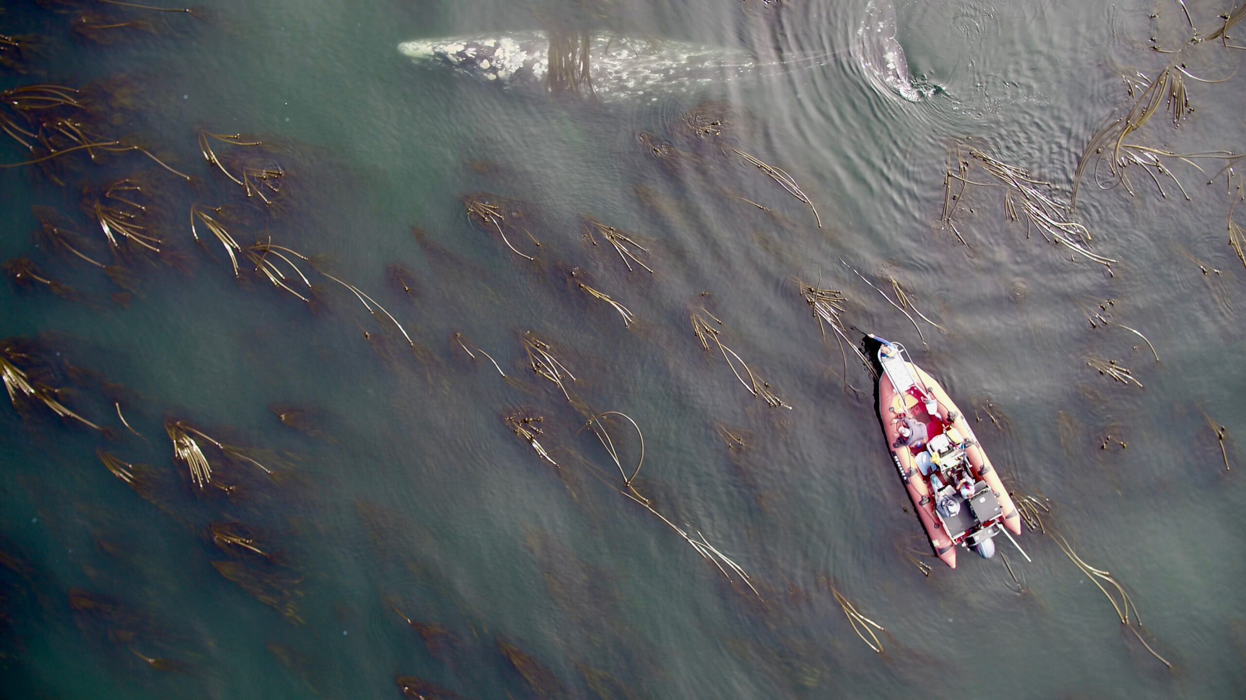
Lunita’s high site fidelity to our study area in 2023 meant that she was an excellent candidate for the suction-cup tagging we have been conducting in the last few years. During suction-cup tagging, we attach a device (or tag) via suction cups to a whale’s back. The tag contains a number of different sensors, including an accelerometer (to measure speed), a gyroscope (to measure direction), and a magnetometer (to measure magnetic field), as well as a high-definition video camera and hydrophone (or underwater microphone). These tags typically stay on for a maximum of 24 hours before they pop off the whale leaving no harm to the whale. Upon retrieval, we can recreate the whale’s dive path and see the environment and conditions that the whale experienced over several hours. We sometimes refer to tagging as giving the gray whales some temporary jewelry because the tags are a very flashy, bright orange color. From the video from Lunita’s tag shows how they soared through kelp forests feeding on mysids for many, many hours. Check out their profile here: https://www.individuwhale.com/whales/lunita/
Burned
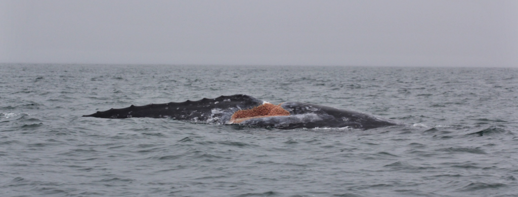
There are many ways to assess the health of a whale. In our lab, we calculate body condition from drone images to determine how fat or skinny a whale is, examine different hormones from their poop, and assess growth rates via length measurements from drone images. Another health assessment metric that we explore in the lab is the skin and scarring on the individuals that we see in our central Oregon study area. By conducting a skin and scarring analysis, we can identify scarring patterns and lesions that may indicate interactions with human activities and track the progression of skin diseases that will help us understand the prevalence and impacts of pathogens on whales. One skin condition that we are particularly interested in tracking appears as a thick white or gray layer that can mask a gray whale’s natural pigmentation. An example of a whale that has experienced this skin condition is “Burned.”

Burned is a female who is at least 9 years old (as of 2024), as she was first documented in the PCFG range in 2015. We saw Burned for the first time in 2016. At the time, we noticed small, isolated, gray patches of the skin condition on both sides of Burned’s body. Throughout the years as we have continued to resight Burned, we noticed the skin condition spreading progressively across her body. We saw the skin condition at its maximum extent in 2022 when, at first glance, Burned was hardly recognizable. Luckily, we can identify gray whales using more than just their pigmentation patterns (learn more on our whale identification page). Interestingly, when we saw Burned in June 2024, it appeared that the skin condition completely disappeared! Burned is just one example of whales with this skin condition, leaving us with many questions about its origin and impact on the whales: What causes the skin condition (viral, fungal, bacterial?); How it is transmitted (via air or contact?); Is it harmful to the whale (weakened immune system?). Our research is aimed at addressing these questions to make this skin condition a little less mysterious. Check out her profile here: https://www.individuwhale.com/whales/burned/
Heart
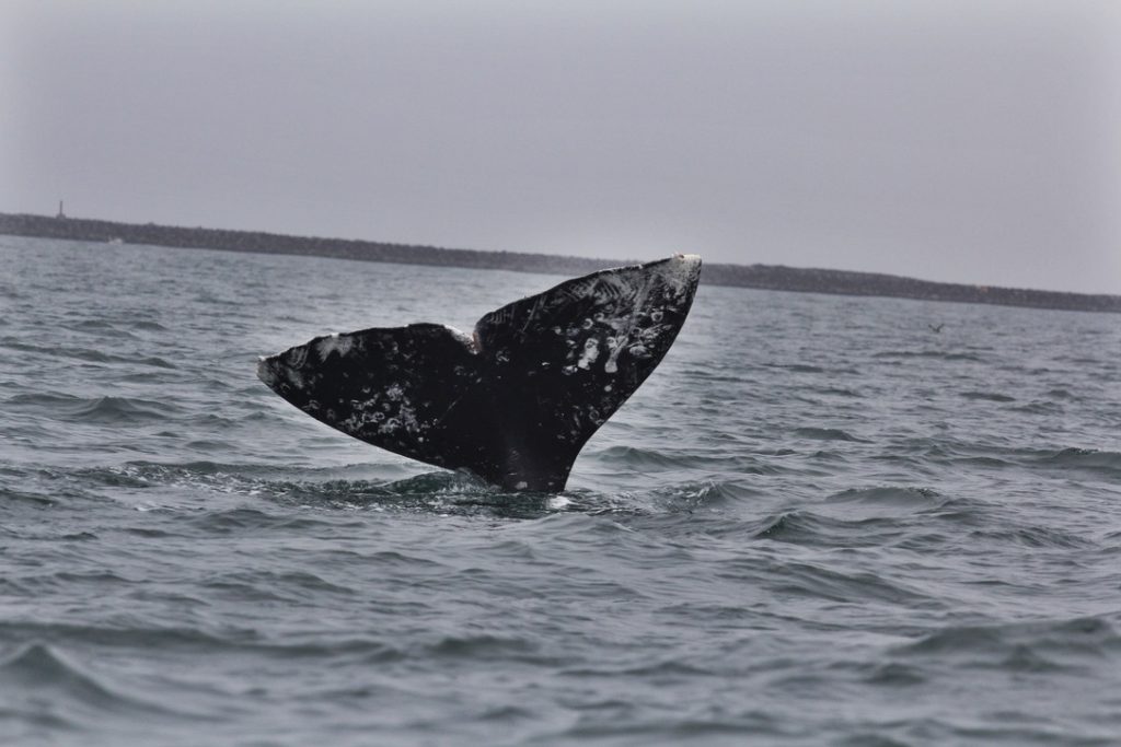
“Heart,” who is also known as “Ginger,” is a very well known and popular whale in the Depoe Bay region. Heart is a female who is particularly famous for being a “tall fluker,” meaning that when she dives, she arches her tail fluke high in the air before it glides elegantly into the water. Heart was first documented as a calf in 2010, which means that she is 14 years old (as of 2024). At 14 years of age, we would expect for Heart to have had at least one, if not more, calves by now, as it is believed that gray whales reach sexual maturity at age 8 or 9. However, Heart has never been documented with a calf. Why?
While we cannot know for sure, we have a theory that it might be linked to her body length. Recent work in our lab has explored how growth of PCFG whales has changed over time. Using measurements of whales from our drone data, we investigated how the asymptotic length (i.e. the final length reached once an individual stops growing) for the PCFG whales has changed since the 1980s. Shockingly, we found that starting in the year 2000 the asymptotic length of PCFG whales has declined at an average rate of 0.05–0.12 meters per year. Over time, this means that a whale born in 2020 is expected to reach an adult body length that is 13% shorter than a gray whale born prior to 2000. In Heart’s case specifically, when we last measured her length at 13 years old, she was 10.65 meters long. If she had been born prior to 2000, then she would be 12.04 meters long by now at the age of 13. That’s a whole 1.5 meters (or almost 5 feet) shorter!

You might be wondering how Heart’s length links back to her ability to have a calf. It takes a lot of energy to be pregnant and support the fetus, so by being smaller, Heart may not be able to store and allocate enough energy towards reproduction. Many of the whales we commonly see are shorter than expected based on their age (including “Zorro”), so we are monitoring the number and frequency of calves in the PCFG to see how this decline in length may impact the population. Check our her profile here: https://www.individuwhale.com/whales/heart/
Be sure to head over to IndividuWhale.com to explore all of the whale profiles and lots of other information that we have provided there about PCFG gray whales and how we study them here in Oregon waters!
Did you enjoy this blog? Want to learn more about marine life, research, and conservation? Subscribe to our blog and get a weekly message when we post a new blog. Just add your name and email into the subscribe box below.