By Lisa Hildebrand, PhD student, OSU Department of Fisheries, Wildlife, & Conservation Sciences, Geospatial Ecology of Marine Megafauna Lab
As I sat down to write this blog, I realized that it is the first post I have written in 2023! This is largely because I have spent the last seven weeks preparing for (and partly taking) my PhD qualifying exams, an academic milestone that involves written and oral exams prepared by each committee member for the student. The point of the qualifying exams is for the student’s committee to determine the student’s understanding of their major field, particularly where and what the limits of that understanding are, and to assess the student’s capability for research. How do you prepare for these exams? Reading. Lots of reading and synthesis of the collective materials assigned by each committee member. My dissertation research covers a broad range of Pacific Coast Feeding Group (PCFG) gray whale ecology, such as space use, oceanography, foraging theory and behavioral responses to anthropogenic activities. Accordingly, my assigned reading lists were equally broad and diverse. For today’s blog, I am going to share some of the papers that have stuck with me and muse about how these topics relate to my study system, the Pacific Coast Feeding Group (PCFG) of gray whales.
Space use & home range
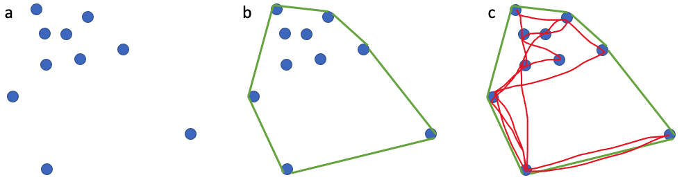
For decades, ecologists have been interested in defining an animal’s use of space through time, often referred to as an animal’s home range. The seminal definition of a home range comes from Burt (1943) who outlined it as “the area traversed by an individual in its normal activities of food gathering, mating, and caring for young.”. I like this definition of a home range because it is biologically grounded and based on an animal’s requirements. However, quantifying an animal’s home range based on this definition is harder than it may sound. In an ideal world, it could be achieved if we were able to collect location data that is continuous (i.e., one location per second), long-term (i.e., at least half the lifespan of an animal) and precise (i.e., correct to the nearest meter) together with behavior for an individual. However, a device that could collect such data, particularly for a baleen whale, does not currently exist. Instead, we must use discontinuous (i.e., one location per hour, day or month) and/or short-term (i.e., <1 year) data with variable precision to calculate animal home ranges. A very common and simple analytical method that is used to calculate an animal’s home range is the minimum convex polygon (MCP). MCP draws the smallest polygon around points with all interior angles less than 180º. While this method is appealing and widely used, it often overestimates the home range by including areas not used by an animal at all (Figure 1).
This example is just one of many where home range estimators inaccurately describe an animal’s space use. However, this does not mean that we should not attempt to make our best approximations of an animal’s home range using the tools and data we have at our disposal. Powell & Mitchell perfectly summarized this sentiment in their 2012 paper: “Understanding animal’s home ranges will be a messy, irregular, complex process and the results will be difficult to map. We must embrace this messiness as it simply represents the real behaviors of animals in complex and variable environments.”. For my second dissertation chapter, I am investigating individual PCFG gray whale space use patterns by calculating activity centers and ranges. The activity center is simply the geographic center of all points of observation (Hayne, 1949) and the range is the distance from the activity center to the most distant point of observations in either poleward direction. While the actual activity center is probably relatively meaningless to a whale, we hope that by calculating these metrics we can identify different strategies of space use that individuals employ to meet their energetic requirements (Figure 2).

Non-stationary responses to oceanography
Collecting spatiotemporally overlapping predator-prey datasets at the appropriate scales is notoriously challenging in the marine environment. As a result, marine ecologists often try to find patterns between marine species and oceanographic and/or environmental covariates, as these can sometimes be easier to sample and thus make marine species predictions simpler. This approach has been applied successfully in hundreds, if not thousands, of studies (e.g., Barlow et al., 2020; Derville et al., 2022). Unfortunately, these relationships are not always proving to be stable over time, a phenomenon called non-stationarity. For example, Schmidt et al. (2014) showed that the reproductive successes of Brandt’s cormorants and Cassin’s auklets on southeast Farallon Island were positively correlated with each other from 1975 to 1995 and were associated with negative El Niño-Southern Oscillation. However, around the mid-1990s this relationship broke down and by 2002, the reproductive successes of the two species were significantly negatively correlated (Figure 3). Furthermore, the relationships between reproductive success and most physical oceanographic conditions became highly variable from year to year and were non-stationary. Thus, if the authors continued to use the relationships defined early on in the study (1975-1995) to predict seabird reproductive success relative to ocean conditions from 2002-2012, their predictions would have been completely wrong. After reading this study, I thought a lot about what the oceanographic conditions have been since the GEMM Lab started studying PCFG gray whales vs. the years prior. Leigh launched the GRANITE project in 2016, right at the tail end of the record marine heatwave in the Pacific, known as “the Blob”. While we do not have as long of a dataset as the Schmidt et al. (2014) study, I wonder whether we might find non-stationary responses between PCFG gray whales and environmental and/or oceanographic variables, given how the effects of the Blob lingered for a long time and we may have captured the central Oregon coast environment shifting from ‘weird to normal’. Non-stationarity is something I will at least keep in mind when I am working on my third dissertation chapter which will investigate the environmental and oceanographic drivers of PCFG gray whale space use strategies.

There are so many more studies and musings that I could write about. I keep being told by others who have been through this qualifying exam process that this is the smartest I am ever going to be, and I finally understand what they mean. After spending almost two months in my own little study world, my research, and where it fits within the complex web of ecological knowledge, has snapped into hyperfocus. I can see clearly where past research will guide me and where I am blazing a new trail of things never attempted before. While I still have the oral portion of my exams before me (in fact, it’s tomorrow!), I am already giddy with excitement to switch back to analyzing data and making progress on my dissertation research.
Did you enjoy this blog? Want to learn more about marine life, research, and conservation? Subscribe to our blog and get a weekly message when we post a new blog. Just add your name and email into the subscribe box below.
References
Barlow, D.R., Bernard, K.S., Escobar-Flores, P., Palacios, D.M., Torres, L.G. 2020. Links in the trophic chain: modeling functional relationships between in situ oceanography, krill, and blue whale distribution under different oceanographic regimes. Marine Ecology Progress Series 642: 207−225.
Burt, W.H. 1943. Territoriality and home range concepts as applied to mammals. Journal of Mammalogy 24(3): 346-352. https://doi.org/10.2307/1374834
Derville, S., Barlow, D.R., Hayslip, C., Torres, L.G. 2022. Seasonal, annual, and decadal distribution of three rorqual whale species relative to dynamic ocean conditions off Oregon, USA. Frontiers in Marine Science 9. https://doi.org/10.3389/fmars.2022.868566
Hayne, D.W. 1949. Calculation of size of home range. Journal of Mammalogy 30(1): 1-18.
Powell, R.A., Mitchell, M.S. 2012. What is a home range? Journal of Mammalogy 93(4): 948-958. https://doi.org/10.1644/11-MAMM-S-177.1
Schmidt, A.E., Botsford, L.W., Eadie, J.M., Bradley, R.W., Di Lorenzo E., Jahncke, J. 2014. Non-stationary seabird responses reveal shifting ENSO dynamics in the northeast Pacific. Marine Ecology Progress Series 499: 249-258. https://doi.org/10.3354/meps10629