The learning curve never stops as the GRANITE project begins its seventh field season

Clara Bird, PhD Student, OSU Department of Fisheries, Wildlife, and Conservation Sciences, Geospatial Ecology of Marine Megafauna Lab

When I thought about what doing fieldwork would be like, before having done it myself, I imagined that it would be a challenging, but rewarding and fun experience (which it is). However, I underestimated both ends of the spectrum. I simultaneously did not expect just how hard it would be and could not imagine the thrill of working so close to whales in a beautiful place. One part that I really did not consider was the pre-season phase. Before we actually get out on the boats, we spend months preparing for the work. This prep work involves buying gear, revising and developing protocols, hiring new people, equipment maintenance and testing, and training new skills. Regardless of how many successful seasons came before a project, there are always new tasks and challenges in the preparation phase.

For example, as the GEMM Lab GRANITE project team geared up for its seventh field season, we had a few new components to prepare for. Just to remind you, the GRANITE (Gray whale Response to Ambient Noise Informed by Technology and Ecology) project’s field season typically takes place from June to mid-October of each year. Throughout this time period the field team goes out on a small RHIB (rigid hull inflatable boat), whenever the weather is good enough, to collect photo-ID data, fecal samples, and drone imagery of the Pacific Coast Feeding Group (PCFG) gray whales foraging near Newport, OR, USA. We use the data to assess the health, ecology and population dynamics of these whales, with our ultimate goal being to understand the effect of ambient noise on the population. As previous blogs have described, a typical field day involves long hours on the water looking for whales and collecting data. This year, one of our exciting new updates is that we are going out on two boats for the first part of the field season and starting our season 10 days early (our first day was May 20th). These updates are happening because a National Science Foundation funded seismic survey is being conducted within our study area starting in June. The aim of this survey is to assess geophysical structures but provides us with an opportunity to assess the effect of seismic noise on our study group by collecting data before, during, and after the survey. So, we started our season early in order to capture the “before seismic survey” data and we are using a two-boat approach to maximize our data collection ability.

While this is a cool opportunistic project, implementing the two-boat approach came with a new set of challenges. We had to find a second boat to use, buy a new set of gear for the second boat, figure out the best way to set up our gear on a boat we had not used before, and update our data processing protocols to include data collected from two boats on the same day. Using two boats also means that everyone on the core field team works every day. This core team includes Leigh (lab director/fearless leader), Todd (research assistant), Lisa (PhD student), Ale (new post-doc), and me (Clara, PhD student). Leigh and Todd are our experts in boat driving and working with whales, Todd is our experienced drone pilot, I am our newly certified drone pilot, and Lisa, Ale, and myself are boat drivers. Something I am particularly excited about this season is that Lisa, Ale, and I all have at least one field season under our belts, which means that we get to become more involved in the process. We are learning how to trailer and drive the boats, fly the drones, and handling more of the post-field work data processing. We are becoming more involved in every step of a field day from start to finish, and while it means taking on more responsibility, it feels really exciting. Throughout most of graduate school, we grow as researchers as we develop our analytical and writing skills. But it’s just as valuable to build our skillset for field work. The ocean conditions were not ideal on the first day of the field season, so we spent our first day practicing our field skills.

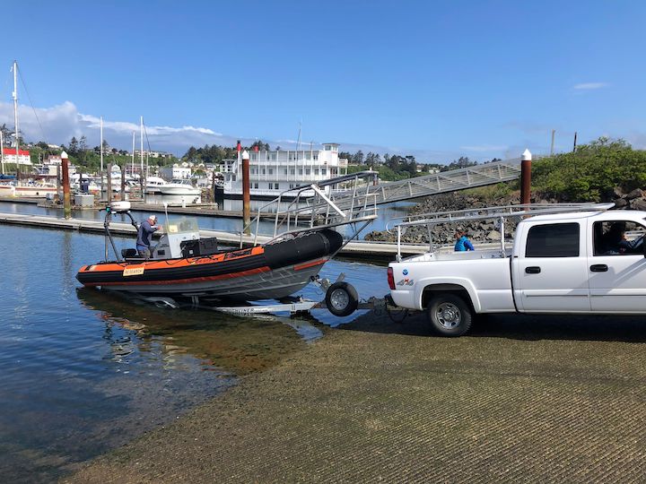
For our “dry run” of a field day, we went through the process of a typical day, which mostly involved a lot of learning from Leigh and Todd. Lisa practiced her trailering and launching of the boat (figure 1), Ale and Lisa practiced driving the boat, and I practiced flying the drone (figure 2). Even though we never left the bay or saw any whales, I thoroughly enjoyed our dry run. It was useful to run through our routine, without rushing, to get all the kinks out, and it also felt wonderful to be learning in a supportive environment. Practicing new skills is stressful to say the least, especially when there is expensive equipment involved, and no one wants to mess up when they’re being watched. But our group was full of support and appreciation for the challenges of learning. We cheered for successful boat launchings and dockings, and drone landings. I left that day feeling good about practicing and improving my drone piloting skills, full of gratitude for our team and excited for the season ahead.

Figure 1. Lisa (driving the truck) launching the boat.
Figure 2. Clara (seated, wearing a black jacket) landing the drone in Ale’s hands.

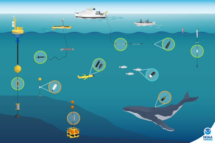
All the diligent prep work paid off on Saturday with a great first day (figure 3). We conducted five GoPro drops (figure 4), collected seven fecal samples from four different whales (figure 5), and flew four drone flights over three individuals including our star from last season, Sole. Combined, we collected two trifectas (photo-ID images, fecal samples, and drone footage)! Our goal is to get as many trifectas as possible because we use them to study the relationship between the drone data (body condition and behavior) and the fecal sample data (hormones). We were all exhausted after 10 hours on the water, but we were all very excited to kick-start our field season with a great day.

Figure 3. Lisa on the bow pulpit during our first sighting of the day.
Figure 4. Lisa doing a GoPro drop, she’s lowering the GoPro into the water using the line in her hands.
Figure 5. Clara and Ale collecting a fecal sample.

On Sunday, just one boat went out to collect more data from Sole after a rainy morning and I successfully flew over her from launching to landing! We have a long season ahead, but I am excited to learn and see what data we collect. Stay tuned for more updates from team GRANITE as our season progresses!

The Road to Oregon

By Imogen Lucciano, incoming graduate student, OSU Department of Fisheries, Wildlife and Conservation Sciences, Geospatial Ecology of Marine Megafauna Lab

There are moments in our individual lifetimes that we can define as noteworthy and right now, as I prepare to start my graduate career within the Marine Mammal Institute (MMI) at OSU, I would say this is it for me. As I sit down to write this blog and document how surreal my future adventure is, I simultaneously feel this path is felicitous. After a year of being cooped up due to COVID, time presently seems to be going by at rocket speed. I am moving constantly in through my day to continue running my current life, while simultaneously arranging all that will encompass my new life. And while I answer questions to my 10-year-old daughter who is doing geometry homework in the living room, while hollering “That is not yours!” to the kitchen where the recently adopted feral dog is sticking his entire head under the trash can lid, while arranging our books in a cardboard box at the packing station I set up on the dining room table, I cannot deny a sense of serenity. This moment in my life, becoming a part of the GEMM Lab and MMI, and relocating to Corvallis is great.

This moment’s noteworthiness is emphasized by embarking on probably the most variable-heavy road trip I have planned to date. Since the age of 19, when I left my small mountain town on the Appalachian trail in Pennsylvania, I have transferred locations ~20 times. Due to extensive travel while serving in the Army (various Army trainings and overseas mission deployments), I have bounced around the US and to other countries often. Over time, one becomes acclimated to the hectic nature of this sort of lifestyle, and yet this new adventure holds significance. 

So here are the details of the adventure trip that lies ahead: I will drive my 2002 Jeep Grand Cherokee across the country; from Charlottesville, Virginia to Corvallis, Oregon. My projected route will extend 2,822 miles and take ~43 driving hours total. The route will fall within the boundaries of 11 states (see Figure 1.)

 Figure 1. Blue Line indicates route from Charlottesville to Corvallis (Google Maps)

Attached to the hitch of the Jeep will be a 6×12 rented cargo trailer containing our treasured books, furniture and things. Inside the Jeep will be three living variables: Mia (the 10-year-old), Angus (hyperactive border collie/ pit bull mix) and Mr. Gibbs (feral pirate dog); all three will need to be closely monitored for potential hiccups in the plan.

If we are going to make it to our destination hotel/Airbnb each night of the trip, I must be organized and calculate road time each day while factoring in breaks to the loo and fueling up. These calculations need to be precise, with little margin for error. I cannot play it too safely either, or it will take us too long to get across the country (I must start my graduate work after all). On the other hand, I cannot realistically expect too many road hours in a day. I think at this point I have got it worked out (Table 1.)

Table 1. Driving Hours and Miles Per Day

When I look back on my career, I had no idea that my not-so-smooth road would lead me to my dream goal of studying marine mammals. I took the Army placement tests at the age of 19, which led me to the field of “information operations” where I earned a great knowledge base in data analysis and encountered fantastic leaders whom I might not have known otherwise. I learned immensely on this path and it set me up very well for moving forward into research and collaboration in the sciences. I am so grateful that my life took this journey because working in the military provided me with the utmost respect for my opportunities and greater empathy for others. This route had many extreme obstacles and was intensely intimidating at times, but I am all the better for it. And I was never able to shake the dream of where I wanted to be (see Figures 2 & 3.) Timing is everything.

Figure 2 & 3. Two of the images of the Pacific coast I have hung up in my house. Keeping my eye on the prize, so to speak. 

It will feel great to cross over the Oregon state line. I cannot wait to meet GEMM Lab in-person and all the other wonderful researchers and staff at MMI and Hatfield Marine Science Center. I am eager to step onto the RV Pacific Storm and begin my thesis research on the magnificent cetaceans off the Oregon coast, and hopefully do some good in the end. As I evaluate the logistics of my trip from Charlottesville to Corvallis, I feel relieved rather than overwhelmed. We could attribute this relief to my not-so-smooth road to get to where I am. Looking ahead, of course, I see a road that will require focus, attention, passion, care, and lots of fuel. Even if this road is not completely smooth, I will have my hands on 10 and 2, and feel so grateful and ready to be on it.

Making predictions: A window into ecological forecast models

By Dawn Barlow, PhD Candidate, OSU Department of Fisheries, Wildlife and Conservation Sciences, Geospatial Ecology of Marine Megafauna Lab

“What is the weather going to be like tomorrow?” “How long will it take to drive there, with traffic?” We all rely on forecasts to make decisions, such as whether to bring a rain jacket, when to get in the car to arrive at a certain destination on time, or any number of situations where we want a prediction of what will happen in the near future. Statistical models underpin many of these examples, using past data to inform future predictions.

Early on in graduate school, I was told that “all models are wrong, but some models work.” Any model is essentially a best approximation, using mathematical relationships, of how we understand a pattern. Models are powerful tools in ecology, enabling us to distill complex, dynamic, and interacting systems into terms and parameters that can be quantified. This ability can help us better understand our study systems and use that understanding to make predictions. We will never be able to describe every nuance of an ecosystem. Instead, the challenge is to collect enough information to build an informed model that can enhance our understanding, without over-simplifying or unnecessarily complicating the system we aim to describe. As Dr. Simon Levin stated in his 1989 seminal paper:

A good model does not attempt to reproduce every detail of the biological system; the system itself suffices for that purpose as the most detailed model of itself. Rather, the objective of a model should be to ask how much detail can be ignored without producing results that contradict specific sets of observations, on particular scales of interest.”1

Species distribution models (SDMs) are the particular branch of models that underpin much of my PhD research on blue whale ecology and distribution in New Zealand. SDMs are mathematical algorithms that correlate observations of a species with environmental conditions at their observed locations to gain ecological insight and predict spatial distributions of the species (Fig. 1)2. The model is a best attempt to quantify and describe the relationships between predictors, e.g., temperature and the observed species distribution pattern. For example, blue whale occurrence is higher in areas of lower temperatures and greater krill availability, and these relationships can be described with models3. So, a model essentially takes all the data available, and synthesizes that information in terms of the relationships between the predictors (environment) and response (species occurrence). Then, we can look at the fitted relationships to ask what we would expect from the species distribution pattern when temperature, or krill availability, or any other predictor, is at a particular value. 

Figure 1. A schematic of a species distribution model (SDM) illustrating how the relationship between mapped species and environmental data (left) is compared to describe “environmental space” (center), and then map predictions from a model using only environmental predictors (right). Note that inter-site distances in geographic space might be quite different from those in environmental space—a and c are close geographically, but not environmentally. The patterning in the predictions reflects the spatial autocorrelation of the environmental predictors. Figure reproduced from Elith and Leathwick (2009).

So, if a model is simply a mathematical description of how terms interact to produce a particular outcome, how do predictions work? To make a spatial prediction, e.g., a map of the probability of a species being present, you need two things: a model describing the functional relationships between species presence and your environmental predictors, and the values of your predictor variables on the day you are interested in predicting to. For example, you may need to obtain a map of sea surface temperature, productivity, temperature anomaly, and surface currents on a day you want to know where whales are expected to be. Your model is the applied across that stack of spatial environmental layers and, based on the functional relationships derived by the model, you get an estimate of the probability of species occurrence based on the temperature, productivity, anomaly, and surface current values at each location. By applying the model over a range of values, you can obtain a continuous surface with the probability of presence, in the form of a map. These maps are typically for the past or present because that is when we can typically acquire spatial environmental layers. However, to make predictions for a future time of interest, we need to have spatial environmental layers for the future.

Forecasts are predictions for the future. Recent advances in technology and computing have led to an emergence of environmental and ecological forecasting tools that are being developed around the world to produce marine forecasts. These tools include predictions of the physical environment such as ocean temperatures or currents, and biological patterns such as where species will be distributed in space and timing of events like salmon spawning or lobster landings4. The ability to generate forecast of marine ecosystems is of particular interest to resource users and managers because it can allow them to be proactive rather than reactive. Forecasts enable us to anticipate events or patterns and prepare, rather than having to respond in real-time or after the fact.

The South Taranaki Bight region in New Zealand is an area where blue whale foraging habitat frequently coincides with industry pressures, including petroleum and mineral extraction, exploration for petroleum reserves using seismic airgun surveys, vessel traffic between ports, and even an ongoing proposal for seabed mining5. Static spatial restrictions to mitigate impacts from these activities on blue whales may be met with resistance from industry user groups, but dynamic spatial management6–8 of blue whale habitat could be more attractive and acceptable. The key for successful dynamic management is knowing where and when to put those boundaries; and this is where ecological forecast models can show their strength. If we can predict suitable blue whale habitat for the future, proactive regulations can be applied to enhance conservation management in the region. Can we develop reliable and useful ecological forecasts for the South Taranaki Bight? Well, given that we have already developed robust models of the relationships between blue whales and their habitat3 and have documented the spatial and temporal lags between wind, upwelling, and blue whales9, we feel confident that we can develop forecast models to predict where blue whales will be in the STB region. As we continue working hard toward this goal, we invite you to check back for our findings in the future. So, consider this blog post a forecast of sorts, and stay tuned!  

Figure 2. A blue whale surfaces in front of an oil extraction platform in the South Taranaki Bight, demonstrating the overlap between whales and industry in the region. Photo by D. Elvines.

References:

1.        Levin, S. A. The problem of pattern and scale. Ecology 73, 1943–1967 (1992).

2.        Elith, J. & Leathwick, J. R. Species Distribution Models: Ecological Explanation and Prediction Across Space and Time. Annu. Rev. Ecol. Evol. Syst. 40, 677–697 (2009).

3.        Barlow, D. R., Bernard, K. S., Escobar-Flores, P., Palacios, D. M. & Torres, L. G. Links in the trophic chain: Modeling functional relationships between in situ oceanography, krill, and blue whale distribution under different oceanographic regimes. Mar. Ecol. Prog. Ser. 642, 207–225 (2020).

4.        Payne, M. R. et al. Lessons from the first generation of marine ecological forecast products. Front. Mar. Sci. 4, 1–15 (2017).

5.        Torres, L. G. Evidence for an unrecognised blue whale foraging ground in New Zealand. New Zeal. J. Mar. Freshw. Res. 47, 235–248 (2013).

6.        Hyrenbach, K. D., Forney, K. A. & Dayton, P. K. Marine protected areas and ocean basin management. Aquat. Conserv. Mar. Freshw. Ecosyst. 10, 437–458 (2000).

7.        Maxwell, S. M. et al. Dynamic ocean management: Defining and conceptualizing real-time management of the ocean. Mar. Policy 58, 42–50 (2015).

8.        Oestreich, W. K., Chapman, M. S. & Crowder, L. B. A comparative analysis of dynamic management in marine and terrestrial systems. Front. Ecol. Environ. 18, 496–504 (2020).

9.        Barlow, D. R., Klinck, H., Ponirakis, D., Garvey, C. & Torres, L. G. Temporal and spatial lags between wind, coastal upwelling, and blue whale occurrence. Sci. Rep. 11, (2021).

Wave riders or deep divers: what do cetaceans do in stormy weather?

By Lisa Hildebrand¹ and Samara Haver²

¹PhD Student, OSU Department of Fisheries, Wildlife, and Conservation Sciences, Geospatial Ecology of Marine Megafauna Lab 

²Postdoctoral Scholar, OSU Department of Fisheries, Wildlife, and Conservation Sciences, Cooperative Institute for Marine Resources Studies, Hatfield Marine Science Center

Many aspects of studying cetacean ecology, behavior, population dynamics, health, and sociality depend on being able to see and/or sample cetaceans when they come to the surface. While this research is not necessarily easy given that cetaceans spend the majority of their time underwater out of human sight, it is definitely feasible, as evidenced by decades of cetacean research. However, in order for researchers to observe cetaceans at the surface they need to get out to sea, and this boat-based effort can realistically only be done in good ocean conditions. Any sea-going individual likely uses the Beaufort sea state (BSS) scale as a measure of ocean conditions. For a full breakdown and excellent explanation of what the BSS is, check out our beloved Alexa’s blog; but for the purposes of this blog all you really need to know is that the smaller the BSS (which starts at 0), the calmer the ocean, and the higher the BSS, the rougher & stormier the ocean. There are two main reasons for conducting cetacean research in low BSS: 1) above a certain threshold (usually BSS 4) it becomes difficult to reliably spot and recognize cetaceans at the surface, thus compromising good data collection, and/or 2) to ensure safety and comfort of the research team. 

So, when the BSS gets too high, us humans usually do not go out to sea to study cetaceans, which means that the cetaceans, for the most part, go unobserved. So, many questions arise about what cetaceans are doing during these rough ocean conditions. What does an increased BSS mean for them? Are they unfazed by big waves and strong winds, or are they affected by the weather and take longer dives or seek out fairer seas? A conversation among friends sparked our curiosity of what cetaceans do in stormy conditions and inspired us to collaborate on this blog. Here, we report on what is and is not known about cetaceans in storms, and discuss some ideas about how best to quantify the effects of rough sea conditions on cetaceans.

Slide the arrows to compare sea conditions (BSS 1 [left] vs BSS 6 [right]) experienced by Alexa, the GEMM Lab marine mammal observer on the May 2019 Northern California Current cruise onboard NOAA ship Bell M. Shimada. Source: A. Kownacki/GEMM Lab.

A literature search of cetaceans during storms did not generate many results, which was not surprising to us given the above reasons about researchers not being able to survey in rough sea conditions. However, we did find a couple of interesting studies about cetacean behavior and distribution after storms.

Changes in foraging behavior

Autumnal storms in Maryland, USA resulted in less frequent and shorter encounters of bottlenose dolphins in the US Mid-Atlantic Bight. However, dolphins spent a significantly higher percentage of their encounters feeding after storms than they did before or during them (Fandel et al. 2020). Similarly, bottlenose dolphins in Mississippi Sound displayed an approximately 15% increase in foraging activity for up to 2 years following Hurricane Katrina (Smith et al. 2013). These changes in foraging behavior are attributed to shifts in distributions and behavior of dolphin prey species as a result of altered environmental conditions (primarily sea surface temperature and salinity) following the hurricanes.

Out-of-habitat events and strandings

An out-of-habitat event occurs when an animal is displaced out of its typical habitat. Seven of these events were reported following Hurricane Rita, which hit the southwest Louisiana coast in 2005, with bottlenose dolphins found in flooded roadside ditches, canals, shallow flooded fields, and a natural creek area (Rosel & Watts 2008). These locations ranged from 2.5 to 11 km inland from the coast of the Gulf of Mexico, where these dolphins were displaced from. It is believed that the animals were carried inland on the storm surge that accompanied Hurricane Rita and were left stranded in areas that held water the longest once it started receding (Rosel & Watts 2008).

One of the roadside ditches where a bottlenose dolphin was trapped in Louisiana following Hurricane Rita. Taken from Rosel & Watts (2008).

There have been two mass strandings of pygmy killer whales that are believed to have been a result of hurricanes. In 1995, five pygmy killer whales stranded (three of which died, while two were successfully refloated) in the British Virgin Islands a day after Hurricane Marilyn (Mignucci-Giannoni et al. 1999). In 2006, six pygmy killer whales (five of which died) stranded in New Caledonia during and after Hurricane Jim (Clua et al. 2014). Both studies hypothesize that increased energetic costs, as a result of attempting to evade the hurricanes, coupled with animals becoming disoriented and ending up in shallow waters, is what caused them to strand. 

While these studies reveal post-storm effects on cetaceans, we still do not know exactly how these individuals behaved during the storms. Did they attempt longer dives to stay away from the rough conditions at the surface, thus becoming disoriented? Or were they behaving normally (i.e. foraging, travelling) and were simply “pushed” into waters that they did not intend to go into? Given that very stormy sea conditions do not allow for visual, boat-based surveys, we need to employ different technologies to study cetacean behavior and distribution during storms.

Passive acoustic monitoring (PAM) is a great tool that can monitor ocean environments for us when the seas are too stormy. Using fixed or mobile platforms, underwater PAM listening devices (hydrophone and data storage) can record sounds in the ocean for us to listen and analyze from shore. With PAM we are able to track the vocalizations of marine mammals as well as other sounds in the environment, such as waves crashing and rain. Anecdotally, we have spent many days at sea in conditions that were too rough for visual observations, but we could safely use our PAM tools to detect cetaceans. So, just because the seas may be too rough to see cetaceans, this fact does not mean that we cannot observe them – we just need to listen instead of look. 

There are many tools that can be used to record underwater sounds, including passive acoustic monitoring (PAM; shown in orange), real-time acoustic data collection (green), and active acoustics (blue.) Source: NOAA Fisheries.

A number of studies have investigated whether whales change their vocalization behavior differently in response to changing ambient sound conditions (for example: Dunlop et al. 2010; Fournet et al. 2018). While research on ocean sound levels is often focused on the impact of human-generated or anthropogenic noise, there are also natural, abiotic sound sources (e.g. wind, rain, ice) that can elevate ambient sound levels. One potential animal response to elevated ambient sound levels is to vocalize at a higher intensity, called the Lombard (or cocktail party) effect. This phenomenon is common for us humans – have you ever been at a party and at some point you realize that you are shouting to someone in order to be heard above the noise of the room? That’s the Lombard effect! Humpback whales in Glacier Bay National Park, Alaska, exhibited the Lombard effect in response to both natural and man-made sounds, but the probability of calling was lower when vessels were present compared to times with only natural sounds (Fournet et al. 2018). It is also possible that whales may vocalize at different frequencies, times, or for shorter durations when the ocean becomes louder, which we can easily track with PAM. Unfortunately, PAM is limited to what we are able to hear, so if we do not hear whales we cannot determine if this result is because their vocalizations are masked by higher intensity sounds, if they stopped vocalizing, or if they left the listening area. 

Animal-borne tags are another kind of autonomous observation tool that could help us understand cetacean behavior and distribution in storms. Admittedly, the logistics of applying tags before an imminent storm are probably complex. However, the development of medium-duration archival tags may provide a good trade-off between deploying tags long enough before a storm begins, thus providing safe working conditions for the research team, while minimizing potential physical impacts to the animals (Szesciorka et al. 2016). There are currently no published tag studies that document cetacean behavior during storms, but a study of a gray-headed albatross, fitted with a satellite transmitter, that successfully foraged during an Antarctic storm (Catry et al. 2004) shows the promise of using animal-borne tags to answer these questions.  

As with many questions about animal behavior, our best option is to combine all of our research tools to piece together evidence about what might be going on in the deep, dark, stormy ocean. Simultaneously collecting acoustic and movement & behavior data through PAM and animal-borne tags, respectively, could allow us to determine how cetaceans behave during storms. While we are probably not poised to tackle these questions right now, perhaps another curious graduate student can take it on for their own PhD research…

References

Catry, P., Phillips, R.A., and J.P. Croxall. Sustained fast travel by a gray-headed albatross (Thalassarchie chrysostoma) riding an Antarctic storm. The Auk 121(4):1208-1213.

Clua, E.E., Manire, C.A., and C. Garrigue. 2014. Biological data of pygmy killer whales (Feresa attenuata) from a mass stranding in New Caledonia (South Pacific) associated with Hurricane Jim in 2006. Aquatic Mammals 40(2):162-172.

Dunlop, R.A., Cato, D.H., and M.J. Noad. 2010. Your attention please: increasing ambient noise levels elicits a change in communication behaviour in humpback whales (Megaptera novaeangliae). Proceedings of the Royal Society B 277(1693):doi.org/10.1098/rspb.2009.2319. 

Fandel, A.D., Garrod, A., Hoover, A.L., Wingfield, J.E., Lyubchich, V., Secor, D.H., Hodge, K.B., Rice, A.N., and H. Bailey. 2020. Effects of intense storm events on dolphin occurrence and foraging behavior. Scientific Reports 10:19247.

Fournet, M.E.H., Matthews, L.P., Gabriele, C.M., Haver, S., Mellinger, D.K., and H. Klinck. 2018. Humpback whales Megaptera novaeangliae alter calling behavior in response to natural sounds and vessel noise. Marine Ecology Progress Series 607:251-268.

Mignucci-Giannoni, A.A., Toyos-González, G. M., Pérez-Padilla, J., Rodríguez-López, M. A., and J. Overing. 1999. Mass stranding of pygmy killer whales (Feresa attenuata) in the British Virgin Islands. Journal of the Marine Biological Association of the United Kingdom 80:759-760.

Rosel, P.E., and H. Watts. 2008. Hurricane impacts on bottlenose dolphins in the northern Gulf of Mexico. Gulf of Mexico Science 25:7.

Smith, C.E., Hurley, B.J., Toms, C.N., Mackey, A.D., Solangi, M., and S.A. Kuczaj II. 2013. Hurricane impacts on the foraging patterns of bottlenose dolphins Tursiops truncatus in Mississippi Sound. Marine Ecology Progress Series 487:231-244.

Szesciorka, A.R., Calambokidis, J., and J.T. Harvey. 2016. Testing tag attachments to increase the attachment duration of archival tags on baleen whales. Animal Biotelemetry 4:18.