
Dr. Enrico Pirotta (CREEM, University of St Andrews) and Dr. Leigh Torres (GEMM Lab, MMI, OSU)
The health of animals affects their ability to survive and reproduce, which, in turn, drives the dynamics of populations, including whether their abundance trends up or down. Thus, understanding the links between health and reproduction can help us evaluate the impact of human activities and climate change on wildlife, and effectively guide our management and conservation efforts. In long-lived species, such as whales, once a decline in population abundance is detected, it can be too late to reverse the trend, so early warning signals are needed to indicate how these populations are faring.
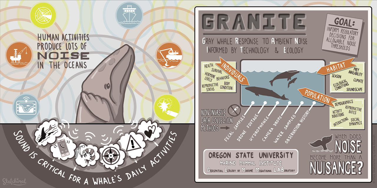
We worked on this complex issue in a study that was recently published in the Journal of Animal Ecology. In this paper, we developed a new statistical approach to link three key components of the health of a Pacific Coast Feeding Group (PCFG) gray whale (namely, its body size, body condition, and stress levels) to a female’s ability to give birth to a calf. We were able to inform these metrics of whale health using an eight-year dataset derived from the GRANITE project of aerial images from drones for measurements of body size and condition, and fecal samples for glucocorticoid hormone analysis as an indicator of stress. We combined these data with observations of females with or without calves throughout the PCFG range over our study period.
We found that for a female to successfully have a calf, she needs to be both large and fat, as these factors indicate if the female has enough energy stored to support reproduction that year (Fig. 1). Remarkably, we also found indication that females with particularly high stress hormone levels may not get pregnant in the first place, which is the first demonstration of a link between stress physiology and vital rates in a baleen whale, to our knowledge.

Our study’s findings are concerning given our previous research indicating that gray whales in this PCFG sub-group have been growing to shorter lengths over the last couple of decades (Pirotta et al. 2023), are thinner than animals in the broader Eastern North Pacific gray whale population (Torres et al, 2022), and show an increase in stress-related hormones when exposed to human activities (Lemos et al, 2022; Pirotta et al. 2023). Furthermore, in our recent study we also documented that there are fewer young individuals than expected for a growing or stable population (Fig. 2), which can be an indicator of a population in decline since there may not be many individuals entering the reproductive adult age groups. Altogether, our results act as early warning signals that the PCFG may be facing a possible population decline currently or in the near future.

These findings are sobering news for Oregon residents and tourists who enjoy watching these whales along our coast every summer and fall. We have gotten to know many of these whales so well – like Scarlett, Equal, Clouds, Lunita, and Pacman, who you can meet on our IndividuWhale website – that we wonder how they will adapt and survive as their once reliable habitat and prey-base changes. We hope our work sparks collective and multifaceted efforts to reduce impacts on these unique PCFG whales, and that we can continue the GRANITE project for many more years to come to monitor these whales and learn from their response to change.
This work exemplifies the incredible value of long-term studies, interdisciplinary methods, and effective collaboration. Through many years of research on this gray whale group, we have collected detailed data on diverse aspects of their behavior, ecology and life history that are critical to understanding their response to disturbance and environmental change, which are both escalating in the study region. We are incredibly grateful to the following members of the PCFG Consortium for contributing sightings and calf observation data that supported this study: Jeff Jacobsen, Carrie Newell, NOAA Fisheries (Peter Mahoney and Jeff Harris), Cascadia Research Collective (Alie Perez), Department of Fisheries and Oceans, Canada (Thomas Doniol-Valcroze and Erin Foster), Mark Sawyer and Ashley Hoyland, Wendy Szaniszlo, Brian Gisborne, Era Horton.
Did you enjoy this blog? Want to learn more about marine life, research, and conservation? Subscribe to our blog and get a weekly alert when we make a new post! Just add your name into the subscribe box below!
References:
Lemos, Leila S., Joseph H. Haxel, Amy Olsen, Jonathan D. Burnett, Angela Smith, Todd E. Chandler, Sharon L. Nieukirk, Shawn E. Larson, Kathleen E. Hunt, and Leigh G. Torres. “Effects of Vessel Traffic and Ocean Noise on Gray Whale Stress Hormones.” Scientific Reports 12, no. 1 (2022): 18580. https://dx.doi.org/10.1038/s41598-022-14510-5.
Pirotta, Enrico, K. C. Bierlich, Leslie New, Lisa Hildebrand, Clara N. Bird, Alejandro Fernandez Ajó, and Leigh G. Torres. “Modeling Individual Growth Reveals Decreasing Gray Whale Body Length and Correlations with Ocean Climate Indices at Multiple Scales.” Global Change Biology 30, no. 6 (2024): e17366. https://doi.org/https://doi.org/10.1111/gcb.17366. https://onlinelibrary.wiley.com/doi/abs/10.1111/gcb.17366.
Pirotta, Enrico, Alejandro Fernandez Ajó, K. C. Bierlich, Clara N Bird, C Loren Buck, Samara M Haver, Joseph H Haxel, Lisa Hildebrand, Kathleen E Hunt, Leila S Lemos, Leslie New, and Leigh G Torres. “Assessing Variation in Faecal Glucocorticoid Concentrations in Gray Whales Exposed to Anthropogenic Stressors.” Conservation Physiology 11, no. 1 (2023). https://dx.doi.org/10.1093/conphys/coad082.
Torres, Leigh G., Clara N. Bird, Fabian Rodríguez-González, Fredrik Christiansen, Lars Bejder, Leila Lemos, Jorge Urban R, et al. “Range-Wide Comparison of Gray Whale Body Condition Reveals Contrasting Sub-Population Health Characteristics and Vulnerability to Environmental Change.” Frontiers in Marine Science 9 (2022). https://doi.org/10.3389/fmars.2022.867258. https://www.frontiersin.org/article/10.3389/fmars.2022.867258


