Migrating south to another foraging ground

By Rachel Kaplan, PhD student, OSU College of Earth, Ocean and Atmospheric Sciences and Department of Fisheries, Wildlife, & Conservation Sciences, Geospatial Ecology of Marine Megafauna Lab 

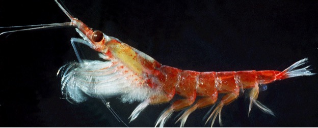
Krill, a shrimplike crustacean found across our oceans, embodies the term “small but mighty”. Though individuals tend to be small, sometimes weighing in at less than a gram, the numerous species of krill have a global distribution and are estimated to collectively outweigh the entire human population. Much of my graduate research focuses on relationships between foraging whales and krill (Euphausia pacifica and Thysanoessa spinifera) in the Northern California Current (NCC) region. This work hinges on themes that are universal across environments: just as krill are ubiquitous across the global ocean, questions of prey quality, distribution, and ecological relationships with predators are universal.

Next week, I’m headed south to consider these questions in a very different foraging environment: the Western Antarctic Peninsula (WAP). One benefit of being a co-advised student is the incredible opportunity to be exposed to diverse projects and types of research. My graduate co-advisor, Kim Bernard, has studied krill in the WAP region for over a decade, and she is currently leading research into the implications of the shifting polar food web for Antarctic krill (Euphasia superba). Through a series of laboratory experiments and fieldwork, the project, titled “The Omnivore’s Dilemma: The effect of autumn diet on winter physiology and condition of juvenile Antarctic krill”,  investigates the impact of climate-driven changes in diet on the health of juvenile krill in autumn and winter, a key time for their survival and recruitment. Winter is a poorly studied season in Antarctica, and this project has already shed light on the physiology, respiration, and growth potential of juvenile krill (Bernard et al., 2022).

 Figure 1: Antarctic krill are much bigger than those found in the NCC region – they can be as long as your thumb! (Source: Australian Antarctic Program)

Just as in the NCC region, krill are an essential link in Southern Ocean food webs, where they transfer energy from their microscopic prey to the higher trophic levels that eat them, including several species of fish, seals, penguins, and whales (Bernard & Steinberg, 2013; Cavan et al., 2019; Ducklow et al., 2013). These predators depend upon this high-quality prey to fuel their seasonal migrations and to build the energy reserves they need to survive the frigid Antarctic winter (Cade et al., 2022; Schaafsma et al., 2018). But, the quality of krill depends upon the food that it can consume itself, and climate change may alter their diet.

There’s a lot to love about krill, but my fascination with them is directly tied to their value as a food source for predators. I want to know how the caloric content of individuals and the aggregations they form changes spatially along the WAP, and how this might shift under climate-forced food web changes. This work will clarify the climate-driven variability in the quality of krill as prey, and the implications this might have for top predators in the region.

Figure 2: The upcoming field season will involve sampling krill along a latitudinal gradient in the WAP region, spanning approximately from the Gerlache Strait in the north to Marguerite Bay in the south (Bernard et al., 2022).

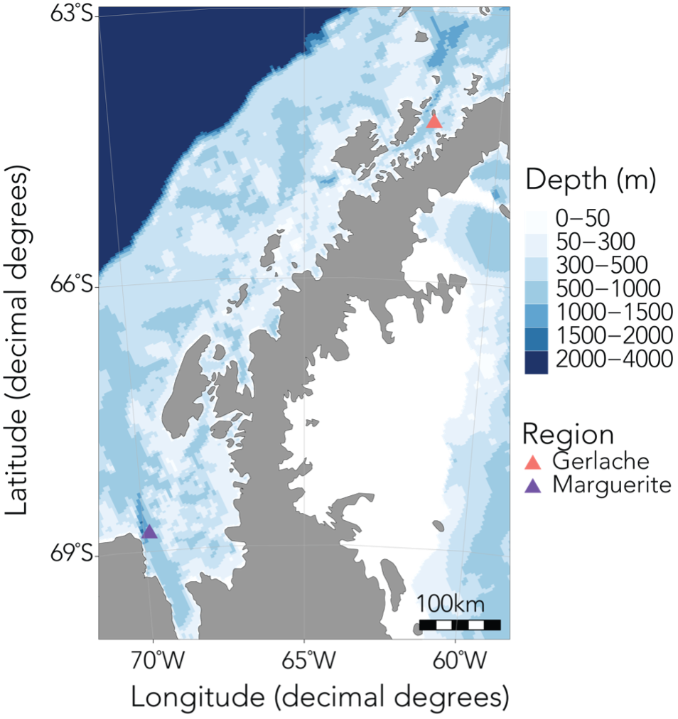
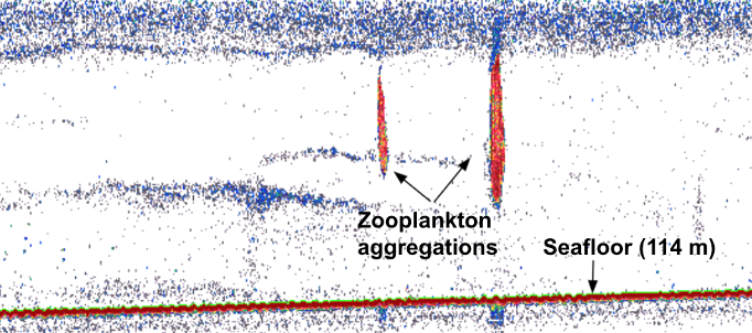
In order to investigate these questions, I’ll be spending the next six months based out of Palmer Station, the smallest of the United States’ research bases in Antarctica, along with Kim and our undergraduate intern Abby. During this upcoming field season, we’ll spend about a month at sea collecting krill samples and active acoustic data using an echosounder, and the rest of the time conducting experiments and sampling in the nearshore. Over the last year, Abby has worked with me to quantify krill caloric content in the NCC, as well as processing samples collected in Antarctica last year. I’m so impressed by everything she’s accomplished, and excited to see her take in this environment, learn a fresh set of experimental and field sampling approaches, and be inspired to ask new questions.

Figure 3: Abby preparing NCC krill samples for caloric analysis (Kim Kenny/OSU CEOAS).

For me, heading south will be a bit like coming home. After graduating from college, I spent about nine months living at Palmer Station and working on the microbial ecology component of the long-term ecological research station there. The experience of being immersed in the WAP environment was foundational to my curiosity about ocean ecology and the impacts of climate change. It is also where I met Kim! All in all, this environment fueled my desire to study krill with Kim and spatial ecology with Leigh, and set me on the course I’m on today.

It also feels meaningful to return here again at this point in my educational journey. With new knowledge and questions I have formed while working in the NCC, I am now excited to apply this knowledge and consider similar questions in the WAP. Abby and I will write blogs through the season and post them here, so stay tuned for news from down south!

Figure 4: Kim and I (the two farthest right in the front row) prepare for a group costumed polar plunge in 2015. Will we do it again? We’ll keep you posted!
Loading

References

Bernard, K. S., & Steinberg, D. K. (2013). Krill biomass and aggregation structure in relation to tidal cycle in a penguin foraging region off the Western Antarctic Peninsula. ICES Journal of Marine Science, 70(4), 834–849. https://doi.org/10.1093/icesjms/fst088

Bernard, K. S., Steinke, K. B., & Fontana, J. M. (2022). Winter condition, physiology, and growth potential of juvenile Antarctic krill. Frontiers in Marine Science, 9, 990853. https://doi.org/10.3389/fmars.2022.990853

Cade, D. E., Kahane-Rapport, S. R., Wallis, B., Goldbogen, J. A., & Friedlaender, A. S. (2022). Evidence for Size-Selective Predation by Antarctic Humpback Whales. Frontiers in Marine Science, 9, 747788. https://doi.org/10.3389/fmars.2022.747788

Cavan, E. L., Belcher, A., Atkinson, A., Hill, S. L., Kawaguchi, S., McCormack, S., Meyer, B., Nicol, S., Ratnarajah, L., Schmidt, K., Steinberg, D. K., Tarling, G. A., & Boyd, P. W. (2019). The importance of Antarctic krill in biogeochemical cycles. Nat Commun, 10(1), 4742. https://doi.org/10.1038/s41467-019-12668-7

Ducklow, H., Fraser, W., Meredith, M., Stammerjohn, S., Doney, S., Martinson, D., Sailley, S., Schofield, O., Steinberg, D., Venables, H., & Amsler, C. (2013). West Antarctic Peninsula: An Ice-Dependent Coastal Marine Ecosystem in Transition. Oceanography, 26(3), 190–203. https://doi.org/10.5670/oceanog.2013.62

Schaafsma, F. L., Cherel, Y., Flores, H., van Franeker, J. A., Lea, M.-A., Raymond, B., & van de Putte, A. P. (2018). Review: The energetic value of zooplankton and nekton species of the Southern Ocean. Marine Biology, 165(8), 129. https://doi.org/10.1007/s00227-018-3386-z

SST, EKE, SSH: Wading Through the Alphabet Soup of Oceanographic Parameters related to Deep-Dwelling Odontocetes

By: Marissa Garcia, PhD Student, Cornell University, Department of Natural Resources and the Environment, K. Lisa Yang Center for Conservation Bioacoustics

Predator-Prey Inference: A Tale as Old as Time

It’s a tale as old as time: where there’s prey, there’ll be predators.

As apex predators, cetaceans act as top-down regulators of ecosystem function. While baleen whales act as “ecosystem engineers,” facilitating nutrient cycling in the ocean (Roman et al., 2014), toothed whales, or “odontocetes,” can impart keystone-level effects — that is, they disproportionately control the marine community’s food-web structure (Valls, Coll, & Christensen, 2015). The menus of prey vary widely by species — ranging from mircronekton to fish to squid – and by extension, vary widely across trophic levels.

So, it naturally follows the old adage: where there’s an abundance of prey, there’ll be an abundance of cetaceans. Yet, creating models that accurately depict this predator-prey relationship is, perhaps unsurprisingly, not as straightforward.

Detecting the ‘Predator’ Half of the Equation

Scientists have successfully documented cetacean presence drawing upon a myriad of methods, each bearing its unique advantages and limitations.

Visual surveys — spanning viewpoints from land, boats, and air — can attain precise spatial data and species ID. However, this data can be constrained by “availability bias” — that is, scientists can only observe cetaceans visible at the surface, not those obscured by the ocean’s depths. Species that spend less time near the surface are more likely to elude the observer’s line of sight, thereby being missed in the data. Consequently, visual surveys have historically undersampled deep-diving species. For instance, since its discovery by western science in 1945, the Hubb’s beaked whale (Mesoplodon carlshubbi) has only been observed alive twice by OSU MMI’s very own Bob Pitman, once in 1994 and another time in 2021.

Scientists have also been increasingly conducting acoustic surveys to document cetacean presence. Acoustic recorders can “hear” each cetacean species at different ranges. Baleen whales, which bellow low-frequency calls, can be heard as far as across ocean basins (Munk et al., 1994). Toothed whales whistle, echolocate, and buzz at frequencies so high they’re considered ultrasonic. But it comes at a trade-off: high-frequency sounds have shorter wavelengths, meaning they are heard across smaller ranges. This high variability, which scientists refer to as “detection range,” translates to not always knowing where the vocalizing cetacean that was recorded is: as such, acoustic data can lack the high-resolution spatial precision often achieved by visual surveys. Nevertheless, acoustic data triumphs in temporal extent, sometimes managing to record continuously at six months at a time. Additionally, animals can elude visual detection in poor weather conditions or if they have a cryptic surface expression, but detected in acoustic surveys (e.g., North Atlantic right whales (Eubalaena glacialis) (Ganley, Brault, & Mayo, 2019; Clark et. al, 2010). Thus, acoustic surveys may be especially optimal for recording elusive deep-dwellers that occupy the often rough Oregon waters, such as beaked whales, the focus of my research in collaboration with the GEMM Lab.

Figure 1: HALO Project researchers Marissa Garcia (left; Yang Center via Cornell) and Imogen Lucciano (right; OSU MMI) among three Rockhopper acoustic recording units, ahead of deployment off the Oregon coast. Credit: Marissa Garcia.

Detecting the ‘Prey’ Half of the Equation

Prey can be measured by numerous methods. Most directly, prey can be measured “in-situ” — that is, prey is collected directly from the site where the cetaceans are detected or observed. A 2020 study combined fish trawls with a towed hydrophone array to identify which fish species odontocetes along the continental shelf of West Ireland (e.g., pilot whales, sperm whales, and Sowerby’s beaked whales) were feasting; the results found that odontocetes primarily fed upon mesopelagic fish and cephalopods (Breen et al., 2020). While trawls can glean species ID of prey, associating this prey data with depth and biomass can prove challenging.

Alternatively, prey can be detected via active acoustics. Echosounders release an acoustic signal that descends through the water column and then echoes back once it hits a sound-scattering organism. Beaked whales forage within deep scattering layers typically composed of myctophid fish and squid, both of which can echo back echosounder pings (Hazen et al., 2011). Thus, echosounder data can map prey density through the water column. When mapping prey density of beaked whales, Hazen et al. 2011 found a strong positive correlation among prey density, ocean vertical structure, and clicks primarily produced while foraging – suggesting beaked whales forage at depth when encountering large, multi-species aggregations of prey.

Figure 2: An example of prey mapping via a Simrad EK60 120 kHz split-beam echosounder. Credit: Rachel Kaplan (OSU MMI) via the HALO Project.

Most relevant to the HALO Project, prey is measured using proximate indices, which are more easily quantifiable metrics of ocean conditions, such as collected from ships via CTD casts or via satellite imagery, that are indirectly related to prey abundance. CTD data can provide information related to the water column structure, including depth and strength of the thermocline, depth of the mixed layer, depth of the euphotic zone, and total chlorophyll concentration in the euphotic zone (Redfern et al. 2006). Satellite imagery can characterize the dynamic patterns of the surface later, including sea surface temperature (SST), salinity, surface chlorophyll a, sea surface height (SSH), and sea surface currents (Virgili et al., 2022; Redfern et al., 2006). Ocean model data products can, such as the Regional Ocean Modeling System (ROMS) which models how an oceanic region of interest responds to physical processes, can provide water column variables related to eddy kinetic energy (EKE) and average temperature gradients (Virgili et al., 2022). In the case of my research with the HALO Project, we will be using oceanographic data collected through the Ocean Observatories Initiative to inform odontocete species distribution models.

Connecting the Dots: Linking Deep-Dwelling Top Predators and Prey

While scientists have made significant advances with collecting both cetacean and prey data, connecting the dots between the ecology of deep-dwelling odontocetes and the oceanographic parameters indicative of their prey still remains a challenge.

In the absence of in situ sampling, species distribution models of marine top predators often derive proxies for “prey data” from static bathymetric and dynamic surface water variables (Virgili et al., 2022). However, surface variables may be irrelevant to toothed whale prey inhabiting great depths (Virgili et al., 2022). Within the HALO Project, the deepest Rockhopper acoustic recording unit is recording odontocetes at nearly 3,000 m below the surface, putting into question the relevance of oceanographic parameters collected at the surface.

Figure 3: Schematic depicting the variation among different zones in the water column. Conditions at the surface may not represent conditions at depth. Credit: Barbara Ambrose, NOAA via NOAA Ocean Explorer.

In my research, I am setting out to estimate which oceanographic variables are optimal for explaining deep-dwelling odontocete presence. A 2022 study using visual survey data found that surface, subsurface, and static variables best explained beaked whale presence, whereas only surface and deep-water variables – not static – best explained sperm whale presence (Virgili et al., 2022). These results are associated with each species’ distinct foraging ecologies; beaked whales may truly only rely on organisms that live near the seabed, whereas sperm whales also feast upon meso-to-bathypelagic organisms, so they may be more sensitive to changes in water column conditions (Virgili et al., 2022). This study expanded the narrative: deep-water variables can also be key to predicting deep-dwelling odontocete presence. The oceanographic variables must be tailored to the ecology of each species of interest.

In the months ahead, I seek to build on this study by investigating which parameters best predict odontocete presence using an acoustic approach instead — I am looking forward to the results to come!

Loading

References

Breen, P., Pirotta, E., Allcock, L., Bennison, A., Boisseau, O., Bouch, P., Hearty, A., Jessopp, M., Kavanagh, A., Taite, M., & Rogan, E. (2020). Insights into the habitat of deep diving odontocetes around a canyon system in the northeast Atlantic ocean from a short multidisciplinary survey. Deep-Sea Research. Part I, Oceanographic Research Papers, 159, 103236. https://doi.org/10.1016/j.dsr.2020.103236

Clark, C.W., Brown, M.W., & Corkeron, P. (2010). Visual and acoustic surveys

for North Atlantic right whales, Eubalaena glacialis, in Cape Cod Bay, Massachusetts, 2001–2005: Management implications. Marine Mammal Science, 26(4), 837-854.

Ganley, L.C., Brault, S., & Mayo, C.A. (2019). What we see is not what there is: Estimating North Atlantic right whale Eubalaena glacialis local abundance. Endangered Species Research, 38, 101-113.

Hazen, E. L., Nowacek, D. P., St Laurent, L., Halpin, P. N., & Moretti, D. J. (2011). The relationship among oceanography, prey fields, and beaked whale foraging habitat in the Tongue of the Ocean. PloS One, 6(4), e19269–e19269.

Munk, W. H., Spindel, R. C., Baggeroer, A., & Birdsall, T. G. (1994). The Heard Island Feasibility Test. The Journal of the Acoustical Society of America, 96(4), 2330–2342. https://doi.org/10.1121/1.410105

Redfern, J. V., Ferguson, M. C., Becker, E. A., Hyrenbach, K. D., Good, C., Barlow, J., Kaschner, K., Baumgartner, M. F., Forney, K. A., Ballance, L. T., Fauchald, P., Halpin, P., Hamazaki, T., Pershing, A. J., Qian, S. S., Read, A., Reilly, S. B., Torres, L., & Werner, F. (2006). Techniques for cetacean–habitat modeling. Marine Ecology. Progress Series (Halstenbek), 310, 271–295.

Roman, J., Estes, J. A., Morissette, L., Smith, C., Costa, D., McCarthy, J., Nation, J., Nicol, S., Pershing, A., & Smetacek, V. (2014). Whales as marine ecosystem engineers. Frontiers in Ecology and the Environment, 12(7), 377–385.

Valls, A., Coll, M., & Christensen, V. (2015). Keystone species: toward an operational concept for marine biodiversity conservation. Ecological Monographs, 85(1), 29–47.

Virgili, A., Teillard, V., Dorémus, G., Dunn, T. E., Laran, S., Lewis, M., Louzao, M., Martínez-Cedeira, J., Pettex, E., Ruiz, L., Saavedra, C., Santos, M. B., Van Canneyt, O., Vázquez Bonales, J. A., & Ridoux, V. (2022). Deep ocean drivers better explain habitat preferences of sperm whales Physeter macrocephalus than beaked whales in the Bay of Biscay. Scientific Reports, 12(1), 9620–9620.

Dealing with uncertainty in ecology and conservation biology

By Dr. Alejandro A. Fernández Ajó, Postdoctoral Scholar, Marine Mammal Institute – OSU Department of Fisheries, Wildlife, & Conservation Sciences, Geospatial Ecology of Marine Megafauna (GEMM) Lab. 

Ecological research focuses on understanding how species and ecosystems interact and function, as well as understanding what drives changes in these interactions and functions over time. Thus, ecology is a critical component of conservation biology. Although uncertainty is present in any research, it is a pervasive characteristic of ecology and conservation biology, often due to our inability to control the complexity of natural systems. Uncertainty poses challenges to decision-making, policy development, and effective conservation strategies, and therefore needs to be understood and addressed when conducting ecological studies and conservation efforts.

There are several sources of uncertainty in ecological research and conservation biology. One of the primary sources arises from incomplete or limited data (epistemic uncertainty). Ecological systems are complex, and obtaining comprehensive data on all relevant variables and scales is often challenging or impossible. Data may be lacking or unavailable for certain species, habitats, or regions, which can hinder the ability to fully understand ecological dynamics and make accurate predictions. Additionally, ecological data may be uncertain or variable due to measurement errors (see blog post), sampling biases, or changes in data collection methods over time (Regan et al. 2002). Furthermore, another source of uncertainty arises from language (linguistic uncertainty). Linguistic uncertainty can result from lack of agreement in the terms and definitions used in the scientific vocabulary (see blog post), which can often result in ambiguous, vague, or context dependent interpretations (Regan et al 2002). These two source-types of uncertainty can create a complex set of challenges.

Uncertainty in ecological research and conservation biology has important implications for decision-making and policy development. When faced with uncertain information, decision-makers may adopt a cautious approach, leading to delayed or ineffective conservation actions. Alternatively, they may make decisions based on incomplete or biased data, which can lead to unintended consequences or wasted resources. Uncertainty can also affect the public’s perception of ecological issues, leading to skepticism, misinformation, or lack of support for conservation initiatives. In addition, uncertainty can also pose challenges in setting conservation priorities. With limited resources, conservation organizations and policymakers must prioritize efforts to protect species or habitats that are at the greatest risk. However, uncertainties in data or predictions can affect the accuracy of risk assessments, leading to potential misallocation of resources. Finally, uncertainty may also arise when assessing the success of conservation interventions, making it difficult to determine the effectiveness of the conservation actions.

Despite the challenges posed by uncertainty, there are ways to address and mitigate its impacts in ecological research and conservation biology. Here are some strategies that the GEMM Lab implements to navigate these nuances in ecological research:

Improving data quality and quantity: Robust data can provide a more accurate understanding of ecological dynamics and facilitate evidence-based decision-making. In this direction, the GEMM Lab develops comprehensive data collection and monitoring efforts that can help reduce uncertainty. The TOPAZ and GRANITE projects, which study gray whale ecology off the Oregon coast, are good examples in this direction due to continuous research efforts since 2015. With these projects we have developed and standardized data collection and analytical methods, improved data accuracy and precision, and are filling knowledge gaps through targeted research.

Emphasizing adaptive management: Adaptive management is an approach that involves learning from ongoing conservation actions and adjusting strategies based on new information (Allen et al. 2015). This approach recognizes that uncertainties are inherent in ecological systems and promotes flexibility in conservation planning. Monitoring and evaluating conservation interventions, and adjusting management strategies, accordingly, can help mitigate the impacts of uncertainty. With OBSIDIAN, OPAL, and HALO projects the GEMM Lab works towards a better understanding of cetaceans’ distribution and its interactions with the oceanographic conditions (e.g., ocean temperature). These research projects can help to forecast the occurrence of whale aggregations and inform management to reduce conflicts when overlapping with human activities. For instance, results from the OPAL project have been incorporated into Dungeness Crab fishing regulations to reduce entanglement risk to whales, and the GEMM Lab is now investigating the effectiveness of these regulations in the SLATE project.

With these projects, along with the many other research efforts conducted by the GEMM lab and the MMI, we are advancing research in marine ecology, through the development and application the best possible science to generate the needed ecological data for effective conservation and management of the marine environment.

Did you enjoy this blog? Want to learn more about marine life, research, and
conservation? Subscribe to our blog and get a weekly message when we post a new
blog. Just add your name and email into the subscribe box below.

Loading

Sources:

Regan, H. M., Colyvan, M., & Burgman, M. A. (2002). A taxonomy and treatment of uncertainty for ecology and conservation biology. Ecological applications, 12(2), 618-628.

Allen, C. R., & Garmestani, A. S. (2015). Adaptive management (pp. 1-10). Springer Netherlands.

https://mmi.oregonstate.edu/gemm-lab/research-projects

https://mmi.oregonstate.edu/gemm-lab/halo-holistic-assessment-living-marine-resources-oregon

https://mmi.oregonstate.edu/gemm-lab/obsidian-observing-blue-whale-spatial-ecology-investigate-distribution-aotearoa-new-zealand

https://mmi.oregonstate.edu/gemm-lab/opal-overlap-predictions-about-large-whales-identifying-co-occurrence-between-whales

https://mmi.oregonstate.edu/gemm-lab/granite-gray-whale-response-ambient-noise-informed-technology-ecology

https://mmi.oregonstate.edu/gemm-lab/topaz-theodolite-overlooking-predators-zooplankton-gray-whale-foraging-ecology

The road to candidacy is paved with knowledge

By Lisa Hildebrand, PhD student, OSU Department of Fisheries, Wildlife, & Conservation Sciences, Geospatial Ecology of Marine Megafauna Lab

As I sat down to write this blog, I realized that it is the first post I have written in 2023! This is largely because I have spent the last seven weeks preparing for (and partly taking) my PhD qualifying exams, an academic milestone that involves written and oral exams prepared by each committee member for the student. The point of the qualifying exams is for the student’s committee to determine the student’s understanding of their major field, particularly where and what the limits of that understanding are, and to assess the student’s capability for research. How do you prepare for these exams? Reading. Lots of reading and synthesis of the collective materials assigned by each committee member. My dissertation research covers a broad range of Pacific Coast Feeding Group (PCFG) gray whale ecology, such as space use, oceanography, foraging theory and behavioral responses to anthropogenic activities. Accordingly, my assigned reading lists were equally broad and diverse. For today’s blog, I am going to share some of the papers that have stuck with me and muse about how these topics relate to my study system, the Pacific Coast Feeding Group (PCFG) of gray whales.

Space use & home range

For decades, ecologists have been interested in defining an animal’s use of space through time, often referred to as an animal’s home range. The seminal definition of a home range comes from Burt (1943) who outlined it as “the area traversed by an individual in its normal activities of food gathering, mating, and caring for young.”. I like this definition of a home range because it is biologically grounded and based on an animal’s requirements. However, quantifying an animal’s home range based on this definition is harder than it may sound. In an ideal world, it could be achieved if we were able to collect location data that is continuous (i.e., one location per second), long-term (i.e., at least half the lifespan of an animal) and precise (i.e., correct to the nearest meter) together with behavior for an individual. However, a device that could collect such data, particularly for a baleen whale, does not currently exist. Instead, we must use discontinuous (i.e., one location per hour, day or month) and/or short-term (i.e., <1 year) data with variable precision to calculate animal home ranges. A very common and simple analytical method that is used to calculate an animal’s home range is the minimum convex polygon (MCP). MCP draws the smallest polygon around points with all interior angles less than 180º. While this method is appealing and widely used, it often overestimates the home range by including areas not used by an animal at all (Figure 1).

Figure 1. (a) 10 point locations where an individual was observed; (b) the home range as determined by the minimum convex polygon method; (c) the red path shows the movements the animal actually took. Note the large white area in (c) where the animal never went even though it is considered part of the animal’s home range.

This example is just one of many where home range estimators inaccurately describe an animal’s space use. However, this does not mean that we should not attempt to make our best approximations of an animal’s home range using the tools and data we have at our disposal. Powell & Mitchell perfectly summarized this sentiment in their 2012 paper: “Understanding animal’s home ranges will be a messy, irregular, complex process and the results will be difficult to map. We must embrace this messiness as it simply represents the real behaviors of animals in complex and variable environments.”. For my second dissertation chapter, I am investigating individual PCFG gray whale space use patterns by calculating activity centers and ranges. The activity center is simply the geographic center of all points of observation (Hayne, 1949) and the range is the distance from the activity center to the most distant point of observations in either poleward direction. While the actual activity center is probably relatively meaningless to a whale, we hope that by calculating these metrics we can identify different strategies of space use that individuals employ to meet their energetic requirements (Figure 2).

Figure 2. Sightings of nine different PCFG individuals across our GRANITE study area. Each circle represents a location where an individual was sighted and circles are color-coded by year. Plotting the raw data of sighting histories of these individuals hints at patterns in space use by different individuals, which I will explore further in my second dissertation chapter.

Non-stationary responses to oceanography

Collecting spatiotemporally overlapping predator-prey datasets at the appropriate scales is notoriously challenging in the marine environment. As a result, marine ecologists often try to find patterns between marine species and oceanographic and/or environmental covariates, as these can sometimes be easier to sample and thus make marine species predictions simpler. This approach has been applied successfully in hundreds, if not thousands, of studies (e.g., Barlow et al., 2020; Derville et al., 2022). Unfortunately, these relationships are not always proving to be stable over time, a phenomenon called non-stationarity. For example, Schmidt et al. (2014) showed that the reproductive successes of Brandt’s cormorants and Cassin’s auklets on southeast Farallon Island were positively correlated with each other from 1975 to 1995 and were associated with negative El Niño-Southern Oscillation. However, around the mid-1990s this relationship broke down and by 2002, the reproductive successes of the two species were significantly negatively correlated (Figure 3). Furthermore, the relationships between reproductive success and most physical oceanographic conditions became highly variable from year to year and were non-stationary. Thus, if the authors continued to use the relationships defined early on in the study (1975-1995) to predict seabird reproductive success relative to ocean conditions from 2002-2012, their predictions would have been completely wrong. After reading this study, I thought a lot about what the oceanographic conditions have been since the GEMM Lab started studying PCFG gray whales vs. the years prior. Leigh launched the GRANITE project in 2016, right at the tail end of the record marine heatwave in the Pacific, known as “the Blob”. While we do not have as long of a dataset as the Schmidt et al. (2014) study, I wonder whether we might find non-stationary responses between PCFG gray whales and environmental and/or oceanographic variables, given how the effects of the Blob lingered for a long time and we may have captured the central Oregon coast environment shifting from ‘weird to normal’. Non-stationarity is something I will at least keep in mind when I am working on my third dissertation chapter which will investigate the environmental and oceanographic drivers of PCFG gray whale space use strategies.

Figure 3. Figure and caption taken from Schmidt et al. (2014).

There are so many more studies and musings that I could write about. I keep being told by others who have been through this qualifying exam process that this is the smartest I am ever going to be, and I finally understand what they mean. After spending almost two months in my own little study world, my research, and where it fits within the complex web of ecological knowledge, has snapped into hyperfocus. I can see clearly where past research will guide me and where I am blazing a new trail of things never attempted before. While I still have the oral portion of my exams before me (in fact, it’s tomorrow!), I am already giddy with excitement to switch back to analyzing data and making progress on my dissertation research.

Did you enjoy this blog? Want to learn more about marine life, research, and conservation? Subscribe to our blog and get a weekly message when we post a new blog. Just add your name and email into the subscribe box below.

Loading

References

Barlow, D.R., Bernard, K.S., Escobar-Flores, P., Palacios, D.M., Torres, L.G. 2020. Links in the trophic chain: modeling functional relationships between in situ oceanography, krill, and blue whale distribution under different oceanographic regimes. Marine Ecology Progress Series 642: 207−225. 

Burt, W.H. 1943. Territoriality and home range concepts as applied to mammals. Journal of Mammalogy 24(3): 346-352. https://doi.org/10.2307/1374834

Derville, S., Barlow, D.R., Hayslip, C., Torres, L.G. 2022. Seasonal, annual, and decadal distribution of three rorqual whale species relative to dynamic ocean conditions off Oregon, USA. Frontiers in Marine Science 9. https://doi.org/10.3389/fmars.2022.868566

Hayne, D.W. 1949. Calculation of size of home range. Journal of Mammalogy 30(1): 1-18. 

Powell, R.A., Mitchell, M.S. 2012. What is a home range? Journal of Mammalogy 93(4): 948-958. https://doi.org/10.1644/11-MAMM-S-177.1

Schmidt, A.E., Botsford, L.W., Eadie, J.M., Bradley, R.W., Di Lorenzo E., Jahncke, J. 2014. Non-stationary seabird responses reveal shifting ENSO dynamics in the northeast Pacific. Marine Ecology Progress Series 499: 249-258. https://doi.org/10.3354/meps10629