SST, EKE, SSH: Wading Through the Alphabet Soup of Oceanographic Parameters related to Deep-Dwelling Odontocetes

By: Marissa Garcia, PhD Student, Cornell University, Department of Natural Resources and the Environment, K. Lisa Yang Center for Conservation Bioacoustics

Predator-Prey Inference: A Tale as Old as Time

It’s a tale as old as time: where there’s prey, there’ll be predators.

As apex predators, cetaceans act as top-down regulators of ecosystem function. While baleen whales act as “ecosystem engineers,” facilitating nutrient cycling in the ocean (Roman et al., 2014), toothed whales, or “odontocetes,” can impart keystone-level effects — that is, they disproportionately control the marine community’s food-web structure (Valls, Coll, & Christensen, 2015). The menus of prey vary widely by species — ranging from mircronekton to fish to squid – and by extension, vary widely across trophic levels.

So, it naturally follows the old adage: where there’s an abundance of prey, there’ll be an abundance of cetaceans. Yet, creating models that accurately depict this predator-prey relationship is, perhaps unsurprisingly, not as straightforward.

Detecting the ‘Predator’ Half of the Equation

Scientists have successfully documented cetacean presence drawing upon a myriad of methods, each bearing its unique advantages and limitations.

Visual surveys — spanning viewpoints from land, boats, and air — can attain precise spatial data and species ID. However, this data can be constrained by “availability bias” — that is, scientists can only observe cetaceans visible at the surface, not those obscured by the ocean’s depths. Species that spend less time near the surface are more likely to elude the observer’s line of sight, thereby being missed in the data. Consequently, visual surveys have historically undersampled deep-diving species. For instance, since its discovery by western science in 1945, the Hubb’s beaked whale (Mesoplodon carlshubbi) has only been observed alive twice by OSU MMI’s very own Bob Pitman, once in 1994 and another time in 2021.

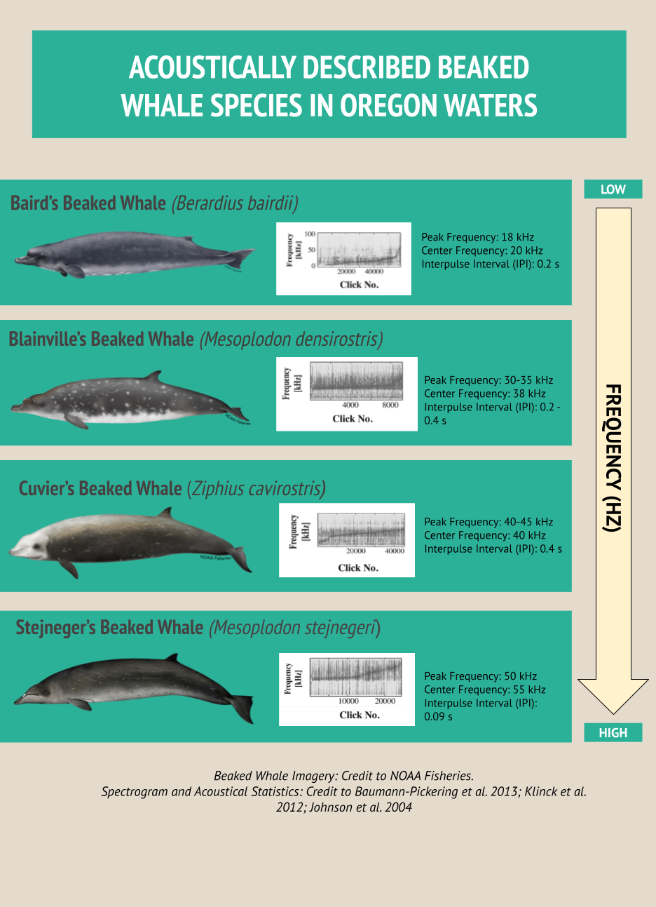
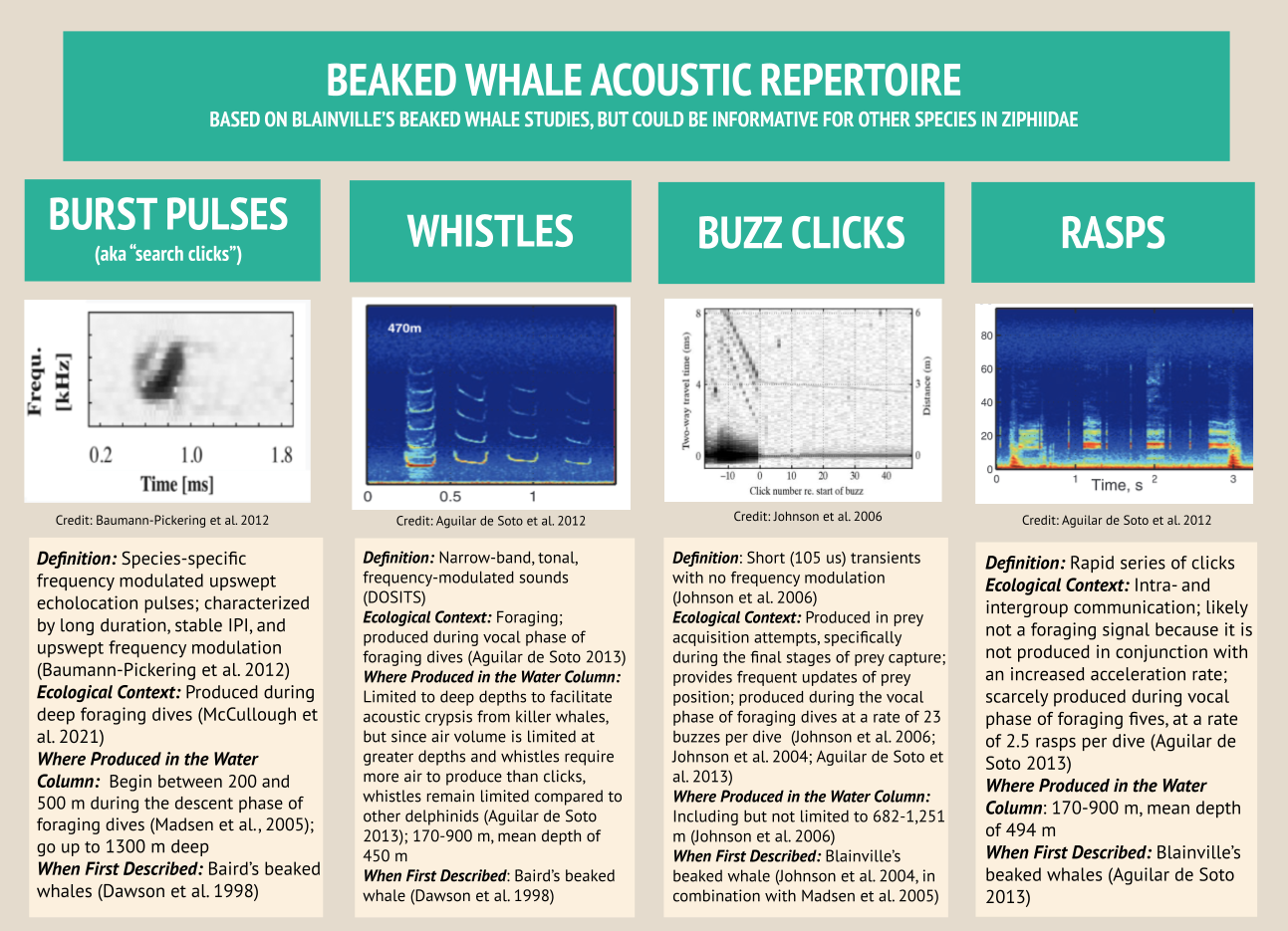
Scientists have also been increasingly conducting acoustic surveys to document cetacean presence. Acoustic recorders can “hear” each cetacean species at different ranges. Baleen whales, which bellow low-frequency calls, can be heard as far as across ocean basins (Munk et al., 1994). Toothed whales whistle, echolocate, and buzz at frequencies so high they’re considered ultrasonic. But it comes at a trade-off: high-frequency sounds have shorter wavelengths, meaning they are heard across smaller ranges. This high variability, which scientists refer to as “detection range,” translates to not always knowing where the vocalizing cetacean that was recorded is: as such, acoustic data can lack the high-resolution spatial precision often achieved by visual surveys. Nevertheless, acoustic data triumphs in temporal extent, sometimes managing to record continuously at six months at a time. Additionally, animals can elude visual detection in poor weather conditions or if they have a cryptic surface expression, but detected in acoustic surveys (e.g., North Atlantic right whales (Eubalaena glacialis) (Ganley, Brault, & Mayo, 2019; Clark et. al, 2010). Thus, acoustic surveys may be especially optimal for recording elusive deep-dwellers that occupy the often rough Oregon waters, such as beaked whales, the focus of my research in collaboration with the GEMM Lab.

Figure 1: HALO Project researchers Marissa Garcia (left; Yang Center via Cornell) and Imogen Lucciano (right; OSU MMI) among three Rockhopper acoustic recording units, ahead of deployment off the Oregon coast. Credit: Marissa Garcia.

Detecting the ‘Prey’ Half of the Equation

Prey can be measured by numerous methods. Most directly, prey can be measured “in-situ” — that is, prey is collected directly from the site where the cetaceans are detected or observed. A 2020 study combined fish trawls with a towed hydrophone array to identify which fish species odontocetes along the continental shelf of West Ireland (e.g., pilot whales, sperm whales, and Sowerby’s beaked whales) were feasting; the results found that odontocetes primarily fed upon mesopelagic fish and cephalopods (Breen et al., 2020). While trawls can glean species ID of prey, associating this prey data with depth and biomass can prove challenging.

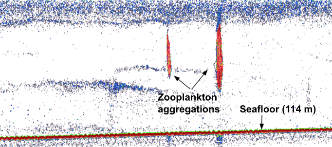
Alternatively, prey can be detected via active acoustics. Echosounders release an acoustic signal that descends through the water column and then echoes back once it hits a sound-scattering organism. Beaked whales forage within deep scattering layers typically composed of myctophid fish and squid, both of which can echo back echosounder pings (Hazen et al., 2011). Thus, echosounder data can map prey density through the water column. When mapping prey density of beaked whales, Hazen et al. 2011 found a strong positive correlation among prey density, ocean vertical structure, and clicks primarily produced while foraging – suggesting beaked whales forage at depth when encountering large, multi-species aggregations of prey.

Figure 2: An example of prey mapping via a Simrad EK60 120 kHz split-beam echosounder. Credit: Rachel Kaplan (OSU MMI) via the HALO Project.

Most relevant to the HALO Project, prey is measured using proximate indices, which are more easily quantifiable metrics of ocean conditions, such as collected from ships via CTD casts or via satellite imagery, that are indirectly related to prey abundance. CTD data can provide information related to the water column structure, including depth and strength of the thermocline, depth of the mixed layer, depth of the euphotic zone, and total chlorophyll concentration in the euphotic zone (Redfern et al. 2006). Satellite imagery can characterize the dynamic patterns of the surface later, including sea surface temperature (SST), salinity, surface chlorophyll a, sea surface height (SSH), and sea surface currents (Virgili et al., 2022; Redfern et al., 2006). Ocean model data products can, such as the Regional Ocean Modeling System (ROMS) which models how an oceanic region of interest responds to physical processes, can provide water column variables related to eddy kinetic energy (EKE) and average temperature gradients (Virgili et al., 2022). In the case of my research with the HALO Project, we will be using oceanographic data collected through the Ocean Observatories Initiative to inform odontocete species distribution models.

Connecting the Dots: Linking Deep-Dwelling Top Predators and Prey

While scientists have made significant advances with collecting both cetacean and prey data, connecting the dots between the ecology of deep-dwelling odontocetes and the oceanographic parameters indicative of their prey still remains a challenge.

In the absence of in situ sampling, species distribution models of marine top predators often derive proxies for “prey data” from static bathymetric and dynamic surface water variables (Virgili et al., 2022). However, surface variables may be irrelevant to toothed whale prey inhabiting great depths (Virgili et al., 2022). Within the HALO Project, the deepest Rockhopper acoustic recording unit is recording odontocetes at nearly 3,000 m below the surface, putting into question the relevance of oceanographic parameters collected at the surface.

Figure 3: Schematic depicting the variation among different zones in the water column. Conditions at the surface may not represent conditions at depth. Credit: Barbara Ambrose, NOAA via NOAA Ocean Explorer.

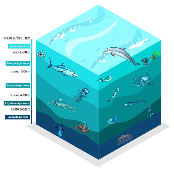
In my research, I am setting out to estimate which oceanographic variables are optimal for explaining deep-dwelling odontocete presence. A 2022 study using visual survey data found that surface, subsurface, and static variables best explained beaked whale presence, whereas only surface and deep-water variables – not static – best explained sperm whale presence (Virgili et al., 2022). These results are associated with each species’ distinct foraging ecologies; beaked whales may truly only rely on organisms that live near the seabed, whereas sperm whales also feast upon meso-to-bathypelagic organisms, so they may be more sensitive to changes in water column conditions (Virgili et al., 2022). This study expanded the narrative: deep-water variables can also be key to predicting deep-dwelling odontocete presence. The oceanographic variables must be tailored to the ecology of each species of interest.

In the months ahead, I seek to build on this study by investigating which parameters best predict odontocete presence using an acoustic approach instead — I am looking forward to the results to come!

Loading

References

Breen, P., Pirotta, E., Allcock, L., Bennison, A., Boisseau, O., Bouch, P., Hearty, A., Jessopp, M., Kavanagh, A., Taite, M., & Rogan, E. (2020). Insights into the habitat of deep diving odontocetes around a canyon system in the northeast Atlantic ocean from a short multidisciplinary survey. Deep-Sea Research. Part I, Oceanographic Research Papers, 159, 103236. https://doi.org/10.1016/j.dsr.2020.103236

Clark, C.W., Brown, M.W., & Corkeron, P. (2010). Visual and acoustic surveys

for North Atlantic right whales, Eubalaena glacialis, in Cape Cod Bay, Massachusetts, 2001–2005: Management implications. Marine Mammal Science, 26(4), 837-854.

Ganley, L.C., Brault, S., & Mayo, C.A. (2019). What we see is not what there is: Estimating North Atlantic right whale Eubalaena glacialis local abundance. Endangered Species Research, 38, 101-113.

Hazen, E. L., Nowacek, D. P., St Laurent, L., Halpin, P. N., & Moretti, D. J. (2011). The relationship among oceanography, prey fields, and beaked whale foraging habitat in the Tongue of the Ocean. PloS One, 6(4), e19269–e19269.

Munk, W. H., Spindel, R. C., Baggeroer, A., & Birdsall, T. G. (1994). The Heard Island Feasibility Test. The Journal of the Acoustical Society of America, 96(4), 2330–2342. https://doi.org/10.1121/1.410105

Redfern, J. V., Ferguson, M. C., Becker, E. A., Hyrenbach, K. D., Good, C., Barlow, J., Kaschner, K., Baumgartner, M. F., Forney, K. A., Ballance, L. T., Fauchald, P., Halpin, P., Hamazaki, T., Pershing, A. J., Qian, S. S., Read, A., Reilly, S. B., Torres, L., & Werner, F. (2006). Techniques for cetacean–habitat modeling. Marine Ecology. Progress Series (Halstenbek), 310, 271–295.

Roman, J., Estes, J. A., Morissette, L., Smith, C., Costa, D., McCarthy, J., Nation, J., Nicol, S., Pershing, A., & Smetacek, V. (2014). Whales as marine ecosystem engineers. Frontiers in Ecology and the Environment, 12(7), 377–385.

Valls, A., Coll, M., & Christensen, V. (2015). Keystone species: toward an operational concept for marine biodiversity conservation. Ecological Monographs, 85(1), 29–47.

Virgili, A., Teillard, V., Dorémus, G., Dunn, T. E., Laran, S., Lewis, M., Louzao, M., Martínez-Cedeira, J., Pettex, E., Ruiz, L., Saavedra, C., Santos, M. B., Van Canneyt, O., Vázquez Bonales, J. A., & Ridoux, V. (2022). Deep ocean drivers better explain habitat preferences of sperm whales Physeter macrocephalus than beaked whales in the Bay of Biscay. Scientific Reports, 12(1), 9620–9620.

Clicks, buzzes, and rasps: How the MMPA has spurred what we know about beaked whale acoustic repertoire

By Marissa Garcia, PhD Student, Cornell University, Department of Natural Resources and the Environment, K. Lisa Yang Center for Conservation Bioacoustics

In October 1972, the tides turned for U.S. environmental politics: the Marine Mammal Protection Act (MMPA) was passed. Its creation ushered in a new flavor of conservation and management. With phrases like “optimum sustainable population” baked into its statutory language, it marked among the first times that ecosystem-based management — an approach which directly calls upon knowledge of ecology to inform action — was required by law (Ray and Potter 2022). Transitioning from reductionist, species-siloed policies, the MMPA instead placed the interdependency of species at the core of ecosystem function and management. 

Beyond deepening the role of science on Capitol Hill, the MMPA’s greatest influence may have been spurred by the language that prohibited “the taking and importation of marine mammals” (16 U.S.C. 1361). Because the word “taking” is multivalent, it carries on its back many interpretations. “Taking” a marine mammal is not limited to intentionally hunting or killing them, or even accidental bycatch. “Taking” also includes carelessly operating a boat when a marine mammal is present, feeding a marine mammal in the wild, or tagging a marine mammal without the appropriate scientific permit. “Taking” a marine mammal can also extend to the fatal consequences caused by noise pollution — not intent, but incident (16 U.S.C. 1362).

The latter circumstances remain reverberant for the U.S. Navy. To comply with the MMPA, they are granted “incidental, but not intentional, taking of small numbers of marine mammals….[when] engag[ing] in a specified activity (other than commercial fishing)” (87 FR 33113). So, if the sonar activities required for national security exercises adversely impact marine mammals, the Navy has a bit of leeway but is still expected to minimize this impact. To further mitigate this potential harm, the Navy thus invests heavily in marine mammal research. (If you are interested in learning more about how the Navy has influenced the trajectory of oceanographic research more broadly, you may find this book interesting.) 

Beaked whales are an example of a marine mammal we know much about due to the MMPA’s call for research when incidental take occurs. Three decades ago, many beaked whales stranded ashore following a series of U.S. Navy sonar exercises. Since then, the Navy has flooded research dollars toward better understanding beaked whale hearing, vocal behavior, and movements (e.g., Klinck et al. 2012). Through these efforts, a deluge of research charged with developing effective tools to acoustically monitor and conserve beaked whales has emerged.  

These studies have laid the foundation for my Ph.D. research, which is dedicated to the Holistic Assessment of Living marine resources off Oregon (HALO) project. Through both visual and acoustic surveys, the HALO project’s mission is to understand how changes in ocean conditions — driven by global climate change — influence living marine resources in Oregon waters. 

In my research specifically, I aim to learn more about beaked whales off the Oregon coast. Beaked whales represent nearly a fourth of cetacean species alive today, with at least 21 species recorded to date (Roman et al. 2013). Even so, 90% of beaked whales are considered data deficient: we lack enough information about them to confidently describe the state of their populations or decide upon effective conservation action. 

Much remains to be learned about beaked whales, and I aim to do so by eavesdropping on them. By referring to the “acoustic repertoire” of beaked whales — that is, their vocalizations and corresponding behaviors — I aim to tease out their vocalizations from the broader ocean soundscape and understand how their presence in Oregon waters varies over time. 

Beaked whales are notoriously cryptic, elusive to many visual survey efforts like those aboard HALO cruises. In fact, some species have only been identified via carcasses that have washed ashore (Moore and Barlow 2013). Acoustic studies have elucidated ecological information (beaked whales forage at night at seamounts summits; Johnston et al. 2008) and have also introduced promising population-level monitoring efforts (beaked whales have been acoustically detected in areas with a historical scarcity of sightings; Kowarski et al. 2018). Their deep-diving nature often renders them inconspicuous, and they forage at depths between 1,000 and 2,000 m, on dives as long as 90 minutes (Moore and Barlow 2013; Klinck et al. 2012). Their echolocation clicks are produced at frequencies within the hearing range of killer whales, and previous studies have suggested that Blainville’s beaked whales are only vocally active during deep foraging dives and not at the surface, possibly to prevent being acoustically detected by predatory killer whales. Researchers refer to this phenomenon as “acoustic crypsis,” or when vocally-active marine mammals are strategically silent to avoid being found by potential predators (Aguilar de Soto et al. 2012).

We expect to see evidence of Blainville’s beaked whales in Oregon waters, as well as Baird’s, Cuvier’s, Stejneger’s, Hubb’s, and other beaked whale species. Species-specific echolocation clicks were comprehensively described a decade ago in Baumann-Pickering et al. 2013 (Figure 1). While this study laid the groundwork for species-level beaked whale acoustic detection, much more work is still needed to describe their acoustic repertoire with higher resolution detail. For example, though Hubb’s beaked whales live in Oregon waters, their vocal behavior remains scantly defined.

Figure 1: Baird’s, Blainville’s, Cuvier’s, and Stejneger’s beaked whales are among the most comprehensively acoustically described beaked whales inhabiting central Oregon waters, though more work would improve accuracy in species-specific acoustic detection. Credit: Marissa Garcia. Infographic draws upon beaked whale imagery from NOAA Fisheries and spectrograms and acoustical statistics published in Baumann-Pickering et al. 2013.

The HALO project seeks to add a biological dimension to the historical oceanographic studies conducted along the Newport Hydrographic (NH) line ever since the 1960s (Figure 2). Rockhopper acoustic recording units are deployed at sites NH 25, NH 45, and NH 65. The Rockhopper located at site NH 65 is actively recording on the seafloor about 2,800 m below the surface. Because beaked whales tend to be most vocally active at these deep depths, we will first dive into the acoustic data on NH 65, our deepest unit, in hopes of finding beaked whale recordings there.

Figure 2: The HALO project team conducts quarterly visual surveys along the NH line, spanning between NH 25 and NH 65. Rockhopper acoustic recording units continuously record at the NH 25, NH 45, and NH 65 sites. Credit: Leigh Torres.

Beaked whales’ acoustic repertoire can be broadly split into four primary categories: burst pulses (aka “search clicks”), whistles, buzz clicks, and rasps. Beaked whale search clicks, which are regarded as burst pulses when produced in succession, have distinct qualities: their upswept frequency modulation (meaning the frequency gets higher within the click), their long duration especially when compared to other delphinid clicks, and a consistent interpulse interval  which is the time of silence between signals (Baumann-Pickering et al. 2013). Acoustic analysts can identify different species based on how the frequency changes in different burst pulse sequences (Baumann-Pickering et al. 2013; Figure 1). For this reason, when I conduct my HALO analyses, I intend to automatically detect beaked whale species using burst pulses, as they are the best documented beaked whale signal, with unique signatures for each species. 

In the landscape of beaked whale acoustics, the acoustic repertoire of Blainville’s beaked whales (Mesoplodon densirostris) — a species of focus in my HALO analyses — is especially well defined. Blainville’s beaked whale whistles have been recorded up to 900 m deep, representing the deepest whistle recorded for any marine mammal to date in the literature (Aguilar de Soto et al. 2012). While Blainville’s beaked whales only spend 40% of their time at depths below 170 m, two key vocalizations occur at these depths: whistles and rasps. While they remain surprisingly silent near the surface, beaked whales produce whistles and rasps at depths up to 900 m. The beaked whales dive together in synchrony, and right before they separate from each other, they produce the most whistles and rasps, further indicating that these vocalizations are used to enhance foraging success (Aguilar de Soto et al. 2006). As beaked whales transition to foraging on their own, they predominantly produce frequently modulated clicks and buzzes. Beaked whales produce buzzes in the final stages of prey capture to receive up-to-date information about their prey’s location. The buzzes’ high repetition enables the whale to achieve 300+ updates on their intended prey’s location in the last 3 m before seizing their feast (Johnson et al. 2006; Figure 3). 

Figure 3: Blainville’s beaked whales generally have four categories within their acoustic repertoire, including burst pulses, whistles, buzz clicks, and rasps. Credit: Marissa Garcia.

All of this knowledge about beaked whale acoustics can be linked back to the MMPA, which has also achieved broader success. Since the MMPA’s implementation, marine mammal population numbers have risen across the board. For marine mammal populations with sufficient data, approximately 65% of these stocks are increasing and 17% are stable (Roman et al. 2013). 

Nevertheless, perhaps much of the MMPA’s true success lies in the research it has indirectly fueled, by virtue of the required compliance of governmental bodies such as the U.S. Navy. And the response has proven to be a boon to knowledge: if the U.S. Navy has been the benefactor of marine mammal research, beaked whale acoustics has certainly been the beneficiary. We hope the beaked whale acoustic analyses stemming from the HALO Project can further this expanse of what we know.

Loading

References

Aguilar de Soto, N., Madsen, P. T., Tyack, P., Arranz, P., Marrero, J., Fais, A., Revelli, E., & Johnson, M. (2012). No shallow talk: Cryptic strategy in the vocal communication of Blainville’s beaked whales. Marine Mammal Science, 28(2), E75–E92. https://doi.org/10.1111/j.1748-7692.2011.00495.x

Baumann-Pickering, S., McDonald, M. A., Simonis, A. E., Solsona Berga, A., Merkens, K. P. B., Oleson, E. M., Roch, M. A., Wiggins, S. M., Rankin, S., Yack, T. M., & Hildebrand, J. A. (2013). Species-specific beaked whale echolocation signals. The Journal of the Acoustical Society of America, 134(3), 2293–2301. https://doi.org/10.1121/1.4817832

Dawson, S., Barlow, J., & Ljungblad, D. (1998). SOUNDS RECORDED FROM BAIRD’S BEAKED WHALE, BERARDIUS BAIRDIL. Marine Mammal Science, 14(2), 335–344. https://doi.org/10.1111/j.1748-7692.1998.tb00724.x

Johnston, D. W., McDonald, M., Polovina, J., Domokos, R., Wiggins, S., & Hildebrand, J. (2008). Temporal patterns in the acoustic signals of beaked whales at Cross Seamount. Biology Letters (2005), 4(2), 208–211. https://doi.org/10.1098/rsbl.2007.0614

Johnson, M., Madsen, P. T., Zimmer, W. M. X., de Soto, N. A., & Tyack, P. L. (2004). Beaked whales echolocate on prey. Proceedings of the Royal Society. B, Biological Sciences, 271(Suppl 6), S383–S386. https://doi.org/10.1098/rsbl.2004.0208

Johnson, M., Madsen, P. T., Zimmer, W. M. X., de Soto, N. A., & Tyack, P. L. (2006). Foraging Blainville’s beaked whales (Mesoplodon densirostris) produce distinct click types matched to different phases of echolocation. Journal of Experimental Biology, 209(Pt 24), 5038–5050. https://doi.org/10.1242/jeb.02596

Klinck, H., Mellinger, D. K., Klinck, K., Bogue, N. M., Luby, J. C., Jump, W. A., Shilling, G. B., Litchendorf, T., Wood, A. S., Schorr, G. S., & Baird, R. W. (2012). Near-real-time acoustic monitoring of beaked whales and other cetaceans using a Seaglider. PloS One, 7(5), e36128. https://doi.org/10.1371/annotation/57ad0b82-87c4-472d-b90b-b9c6f84947f8

Kowarski, K., Delarue, J., Martin, B., O’Brien, J., Meade, R., Ó Cadhla, O., & Berrow, S. (2018). Signals from the deep: Spatial and temporal acoustic occurrence of beaked whales off western Ireland. PloS One, 13(6), e0199431–e0199431. https://doi.org/10.1371/journal.pone.0199431

Madsen, P. T.,  Johnson, M., de Soto, N. A., Zimmer, W. M. X., & Tyack, P. (2005). Biosonar performance of foraging beaked whales (Mesoplodon densirostris). Journal of Experimental Biology, 208(Pt 2), 181–194. https://doi.org/10.1242/jeb.01327

McCullough, J. L. K., Wren, J. L. K., Oleson, E. M., Allen, A. N., Siders, Z. A., & Norris, E. S. (2021). An Acoustic Survey of Beaked Whales and Kogia spp. in the Mariana Archipelago Using Drifting Recorders. Frontiers in Marine Science, 8. https://doi.org/10.3389/fmars.2021.664292

Moore, J. E. & Barlow, J. P. (2013). Declining abundance of beaked whales (family Ziphiidae) in the California Current large marine ecosystem. PloS One, 8(1), e52770–e52770. https://doi.org/10.1371/journal.pone.0052770

Ray, G. C. & Potter, F. M. (2011). The Making of the Marine Mammal Protection Act of 1972. Aquatic Mammals, 37(4), 522.

Roman, J., Altman, I., Dunphy-Daly, M. M., Campbell, C., Jasny, M., & Read, A. J. (2013). The Marine Mammal Protection Act at 40: status, recovery, and future of U.S. marine mammals. Annals of the New York Academy of Sciences, 1286(1), 29–49. https://doi.org/10.1111/nyas.12040

Coastal oceanography takes patience

Joe Haxel, Acoustician, Assistant Professor, CIMRS/OSU

Greetings GEMM Lab blog readers. My name is Joe Haxel and I’m a close collaborator with Leigh and other GEMM lab members on the gray whale ecology, physiology and noise project off the Oregon coast. Leigh invited me for a guest blog appearance to share some of the acoustics work we’ve been up to and as you’ve probably guessed by now, my specialty is in ocean acoustics. I’m a PI in NOAA’s Pacific Marine Environmental Laboratory’s Acoustics Program and OSU’s Cooperative Institute for Marine Resources Studies where I use underwater sound to study a variety of earth and ocean processes.

As a component of the gray whale noise project, during the field seasons of 2016 and 2017 we recorded some of the first measurements of ambient sound in the shallow coastal waters off Oregon between 7 and 20 meters depth. In the passive ocean acoustics world this is really shallow, and with that comes all kinds of instrument and logistical challenges, which is probably one of the main reasons there is little or no acoustic baseline information in this environment.

For instance, one of the significant challenges is rooted in the hydrodynamics surrounding mobile recording systems like the drifting hydrophone we used during the summer field season in 2016 (Fig 1). Decoupling motion of the surface buoy (e.g., caused by swell and waves) from the submerged hydrophone sensor is critical, and here’s why. Hydrophones convert pressure fluctuations at the sensor/ water interface to a calibrated voltage recorded by a logging system. Turbulence resulting from moving the sensor up and down in the water column with surface waves introduces non-acoustic pressure changes that severely contaminate the data for noise level measurements. Vertical and horizontal wave motions are constantly acting on the float, so we needed to engineer compliance between the surface float and the suspended hydrophone sensor to decouple these accelerations. To overcome this, we employed a couple of concepts in our drifting hydrophone design. 1) A 10 cm diameter by 3 m long spar buoy provided floatation for the system. Spar buoys are less affected by wave motion accelerations compared to most other types of surface floatation with larger horizontal profiles and drag. 2) A dynamic shock cord that could stretch up to double its resting length to accommodate vertical motion of the spar buoy; 3) a heave plate that significantly reduced any vertical motion of the hydrophone suspended below it. This was a very effective design, and although somewhat cumbersome in transport with the RHIB between deployment sites, the acoustic data we collected over 40 different drifts around Newport and Port Orford in 2016 was clean, high quality and devoid of system induced contamination.

Figure 1. The drifting hydrophone system used for 40 different drifts recording ambient noise levels in 7-20 m depths in the Newport and Port Orford, OR coastal areas.


Spatial information from the project’s first year acoustic recordings using the drifting hydrophone system helped us choose sites for the fixed hydrophone stations in 2017. Now that we had some basic information on the spatial variability of noise within the study areas we could focus on the temporal objectives of characterizing the range of acoustic conditions experienced by gray whales over the course of the entire foraging season at these sites in Oregon. In 2017 we deployed “lander” style instrument frames, each equipped with a single, omni-directional hydrophone custom built by Haru Matsumoto at our NOAA/OSU Acoustics lab (Fig. 2). The four hydrophone stations were positioned near each of the ports (Yaquina Bay and Port Orford) and in partnership with the Oregon Department of Fish and Wildlife Marine Reserves program in the Otter Rock Marine Reserve and the Redfish Rocks Marine Reserve. The hydrophones were programmed on a 20% duty cycle, recording 12 minutes of every hour at 32 kHz sample rate, providing spectral information in the frequency band from 10 Hz up to a 13 kHz.

Figure 2. The hydrophone (black cylinder) on its lander frame ready for deployment.

Here’s where the story gets interesting. In my experience so far putting out gear off the Oregon coast, anything that has a surface expression and is left out for more than a couple of weeks is going to have issues. Due to funding constraints, I had to challenge that theory this year and deploy 2 of the units with a surface buoy. This is not typically what we do with our equipment since it usually stays out for up to 2 years at a time, is sensitive, and expensive. The 2 frames with a surface float were going to be deployed in Marine Reserves far enough from the traffic lanes of the ports and in areas with significantly less traffic and presumably no fishing pressure.  The surface buoy consisted of an 18 inch diameter hard plastic float connected to an anchor that was offset from the instrument frame by a 150 foot weighted groundline. The gear was deployed off Newport in June and Port Orford in July. What could go wrong?

After monthly buoy checks by the project team, including GPS positions, and buoy cleanings my hopes were pretty high that the surface buoy systems might actually make it through the season with recoveries scheduled in mid-October. Had I gambled and won? Nope. The call came in September from Leigh that one of the whale watching outfits in Depoe Bay recovered a free floating buoy matching ours. Bummer. Alternative recovery plans initiated and this is where things began to get hairy. Fortunately, we had an ace in our back pocket. We have collaborators at the Oregon Coast Aquarium (OCA) who have a top-notch research diving team led by Jim Burke. In the last week of October, they performed a successful search dive on the missing unit near Gull Rock and attached a new set of floats directly to the instrument frame. The divers were in the water for a short 20 minutes thanks to the good series of marks recorded during the buoy checks throughout the summer (Fig. 3).

Figure 3. OCA divers, Jenna and Doug, heading out for a search dive to locate and mark the Gull Rock hydrophone lander.


We had surface marker floats on the frame, but there was a new problem. Video taken by Jenna and Doug from the OCA dive team revealed the landers were pretty sanded in from a couple of recent October storms (Fig. 4). Ugghhh!

Figure 4. Sanded in lander at Gull Rock. Notice the sand dollars and bull kelp wrapped on the frame.

Alternative recovery plan adjustment: we’re gonna need a diver assisted recovery with 2 boats. One to bring a dive team to air jet the sand out away from the legs of the frame and another larger vessel with pulling power to recover the freed lander. Enter the R/V Pacific Surveyor and Capt. Al Pazar. Al, Jim and I came up with a new recovery plan and only needed a decent weather window of a few hours to get the job done. Piece of cake in November off the Oregon coast, right?

The weather finally cooperated in early December in-line with the OCA dive team and R/V Pacific Surveyor’s availability. The 2 vessels and crew headed up to Gull Rock for the first recovery operation of the day. At first we couldn’t locate the surface floats. Oh no. It seemed the rough fall/ winter weather and high seas since late October were too much for the crab floats? As it turns out, we eventually found the floats eastward about 200 m but couldn’t initially see them in the glare and whitecapping conditions that morning. The lander frame had broken loose from its weakened anchor legs in the heavy weather (as it was designed to do through an Aluminum/ Stainless Steel galvanic reaction over time) and rolled or hopped eastward by about 200 m (Fig. 5). Oh dear!

Figure 5. A hydrophone lander after recovery. Notice all but 1 of the concrete anchor legs missing from the recovered lander and the amount of bio-fouling on the hydrophone (compared to Figure 2).


Thankfully, the hydrophone was well protected, and no air jetting was required. With OCA divers out of the water and clear, the Pacific Surveyor headed over to the floats and easily pulled the lander frame and hydrophone on board (Fig. 6). Yipee!

On to the next hydrophone station. This station, deployed ~ 800 m west of the south reef off of South Beach near the Yaquina Bay port entrance. It was deployed entirely subsurface and was outfitted with an acoustic release transponder that I could communicate with from the surface and command to release a pop-up messenger float and line for eventual recovery of the instrument frame. Once on station, communication with the release was established easily (a good start) and we began ranging and moving the OCA vessel Gracie Lynn in to a position within about 2 water depths of the unit (~40 m). I gave the command to the transponder and the submerged release confirmed it was free of its anchor and heading for the surface, but it never made it. Uh oh. Turns out this lander had also broke free of its anchored legs and rolled/ hopped 800 m eastward until it was pinned up against the boulder structure of the south reef. Amazingly, OCA divers Jenna and Doug located the messenger float ~ 5 m below the surface and the messenger line had been fouled by the rolling frame so it could not reach the surface. They dove down the messenger line and attached a new recovery line to the lander frame and the Pacific Surveyor hauled up the frame and hydrophone in-tact (Fig. 6). Double recovery success!

Figure 6. R/V Pacific Surveyor recovering hydrophone landers off Gull Rock and South Beach.

The hydrophone data from both systems looks outstanding and analysis is underway. This recovery effort took a huge amount of patience and the coordination of 3 busy groups (NOAA/OSU, OCA, Capt. Al). Thanks to these incredible collaborations and some heroic diving from Jim Burke and his OCA dive team, we now have a unique and unprecedented shallow water passive acoustic data set from the energetic waters off the Oregon coast.

So that’s some of the story from the 2016 and 2017 field season acoustic point of view. I’ll save the less exciting, but equally successful instrument recoveries from Port Orford for another time.

SeaBASS 2016

By Samara Haver, MSc student, OSU Fisheries and Wildlife, ORCAA Lab

As a graduate student in bioacoustics (the study of noise produced by biological sources), my education is interdisciplinary. Bioacoustics is a relatively small field, and (together with my peers) I am challenged to find my way through coursework in ecology, physiology, physics, oceanography, statistics, and engineering to learn the background information that I need to develop and answer research questions (since this is my first post for the GEMM lab, here is a little more information about my interests). While this challenge (for all young bioacousticians) presents itself a little differently at all universities, the information gap is essentially the same. Hence, just over 6 years ago, Dr. Jennifer Missis-Old and Dr. Susan Parks recognized a need to fill this gap for graduate students in bioacoustics and created SeaBASS, a BioAcoustics Summer School.

This year, for the 4th iteration of the week-long program, I was lucky to have the opportunity to attend SeaBASS. I first heard about SeaBASS as a research assistant in Dr. Sofie Van Parijs’s passive acoustics group at the Northeast Fisheries Science Center, but the workshop is limited to graduate students only so I had to wait until I was officially enrolled in grad school to apply. My ORCAA lab-mates, Niki, Selene, and Michelle are all alumni of SeaBASS (read Miche’s re-cap from 2014 here ) so by the time I was preparing for my trip to upstate NY this summer to attend, I had a pretty good idea of what was to come.

As expected, the week was packed. I flew to the East Coast a few days early to visit our fearless ORCAA leader, Holger, at the Bioacoustics Research Program at the Cornell Lab of Ornithology, so I was lucky to be somewhat adjusted to EST by the time I arrived at Syracuse on Sunday afternoon. After exploring the campus, it was time for official SeaBASS programming to begin. Our first class, an “Introduction to Acoustics and Proportion”, began early on Monday morning. In the afternoon and through the rest of the week we also learned about active acoustics (creating a sound in the water and using the echo to detect animals or other things) and marine mammal physiology, echolocation, communication, and behavior. We also heard about passive acoustics (listening to existing underwater sounds), including the different types of technology being used and its application for population density estimation. On Friday afternoon, the final lecture covered the effects of noise on marine mammals.

Samara1 Some SeaBASS-ers testing the hypothesis that humans are capable of echolocation.

In addition to the class lectures given by each instructor, we also heard individual opinions about “hot topics” in bioacoustics. This session was my favorite part of the week because we (the students) had the opportunity to hear from a number of accomplished scientists about what they believe are the most pressing issues in the field. Unlike a conference or seminar, these short talks introduced (or reinforced) ideas from researchers in an informal setting, and among our small group it was easy to hear impressions from other SeaBASS-ers afterwards. As a student I spend a lot of my time working alone; my ORCAA labmates are focused on related acoustic projects, but we do not overlap completely. The best part of SeaBASS was sharing ideas, experiences, and general camaraderie with other students that are tackling questions very similar to my own.

Samara2 SeaBASS 2016

Although a full week of class would be plenty to take in by itself, our evenings were also filled with activities. We (students) shared posters (this was mine ) about our individual research projects, listened to advice about life as a researcher in the field, attended a Syracuse Chiefs baseball game, and at the end of each day reflected on our new knowledge and experiences over pints. So, needless to say, I returned home to Oregon completely exhausted, but also with refreshed excitement about my place in the small world of bioacoustics research.

Samara3 Luckily we had beautiful weather for the baseball game!

Samara4