By Dawn Barlow, PhD Candidate, OSU Department of Fisheries, Wildlife, and Conservation Sciences, Geospatial Ecology of Marine Megafauna Lab
In human cultures, how you sound is often an indicator of where you are from. Have you ever taken a linguistics quiz that tries to guess what part of the United States you grew up in? Questions about whether you pronounce the sugary sweet treat caramel as “carr-mul” or “care-a-mel”, whether you say “soda” or “pop”, or whether a certain type of intersection is called a “roundabout”, “rotary”, or “traffic circle” are used to make a guess at where in the country you were raised. I have spent time in the United States, Australia, and New Zealand, I was amused to learn that the shoes you might wear in summertime can be called flip flops, slippers, thongs, or jandals, depending on which English-speaking country you are in. We know that listening to how someone speaks can tell us about their heritage or culture. As it turns out, the same is true for blue whales. We can learn a lot about blue whales by listening to them.

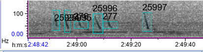
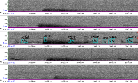
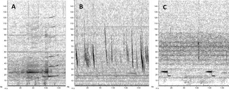
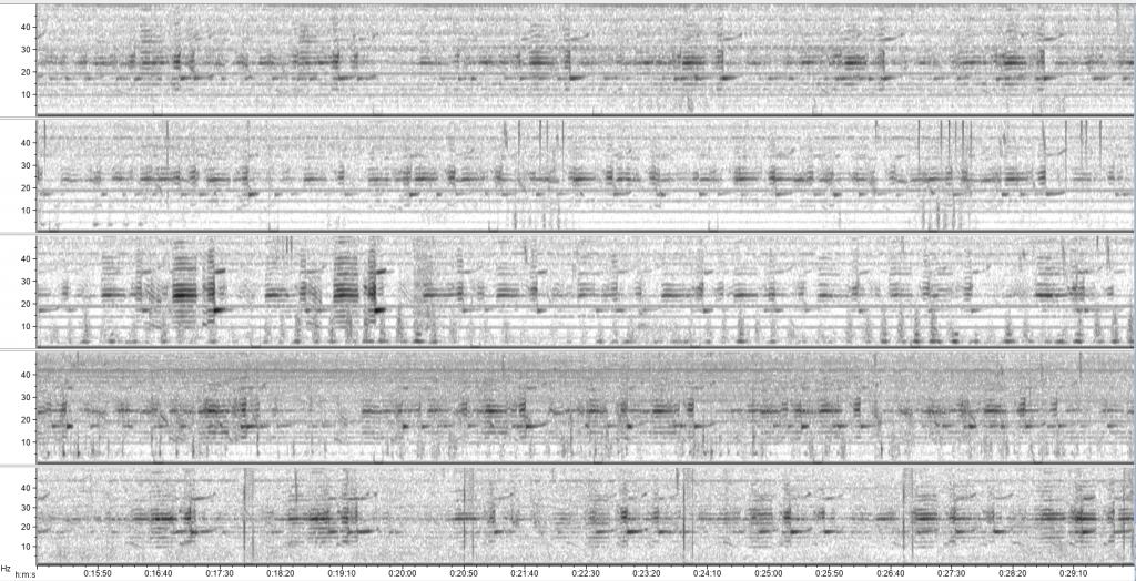
Sound is an incredibly important sense to marine mammals, particularly since sound waves can efficiently transmit over long distances in the ocean where other senses, such as vision or smell, are limited. Therefore, passive acoustic monitoring—placing hydrophones underwater to listen for an extended period of time and record the sounds of animals and their environment—is a highly effective tool for studying marine mammals, including blue whales. Throughout the world, blue whales sing. In this case, “song” is defined as a limited number of sound types that are produced in succession to form a recognizable pattern (McDonald et al. 2006). These songs are presumed to be produced by males only, most likely used to maintain associations and mediate social interactions, and seem to play a role in reproduction (Oleson et al. 2007, Lewis et al. 2018). Furthermore, these songs are highly stereotyped, and stable over decadal scales (McDonald et al. 2006).
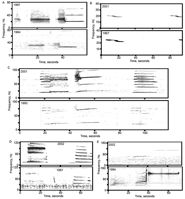
Fascinatingly, blue whale songs have acoustic characteristics that are distinct between geographic regions. A blue whale in the northeast Pacific sings a different song than a blue whale in the north Atlantic; the song heard around Australia is distinct from the one sung off the coast of Chile, and so on. Therefore, differences in blue whale songs between areas can be used as a provisional hypothesis about population structure (McDonald et al. 2006, Samaran et al. 2013, Balcazar et al. 2015). Vocalizations may evolve more rapidly than traditional markers such as genetics or morphology that are often used to delineate populations, particularly in long-lived mammalian species such as blue whales (McDonald et al. 2006).

Despite the general rule of thumb that population-specific blue whale songs occur in separate geographic regions, there are examples throughout the southern hemisphere where songs from different populations overlap and are recorded in the same location (Samaran et al. 2010, 2013, Tripovich et al. 2015, McCauley et al. 2018, Buchan et al. 2020, Leroy et al. 2021). However, these examples may be instances where the populations temporally or ecologically partition their use of the area. For example, there may be differences in the timing of peak occurrence so that overlap is minimized by alternating which population is predominantly present in different seasons (Leroy et al. 2018). Alternatively, whales from different populations may overlap in space and time, but occupy different ecological niches at the same site. In this case, an area may simultaneously be a migratory corridor for one population and a foraging ground for another (Tripovich et al. 2015).
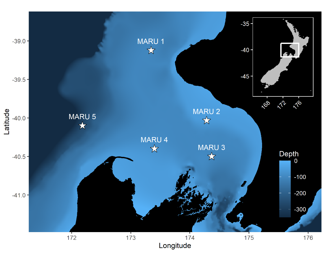
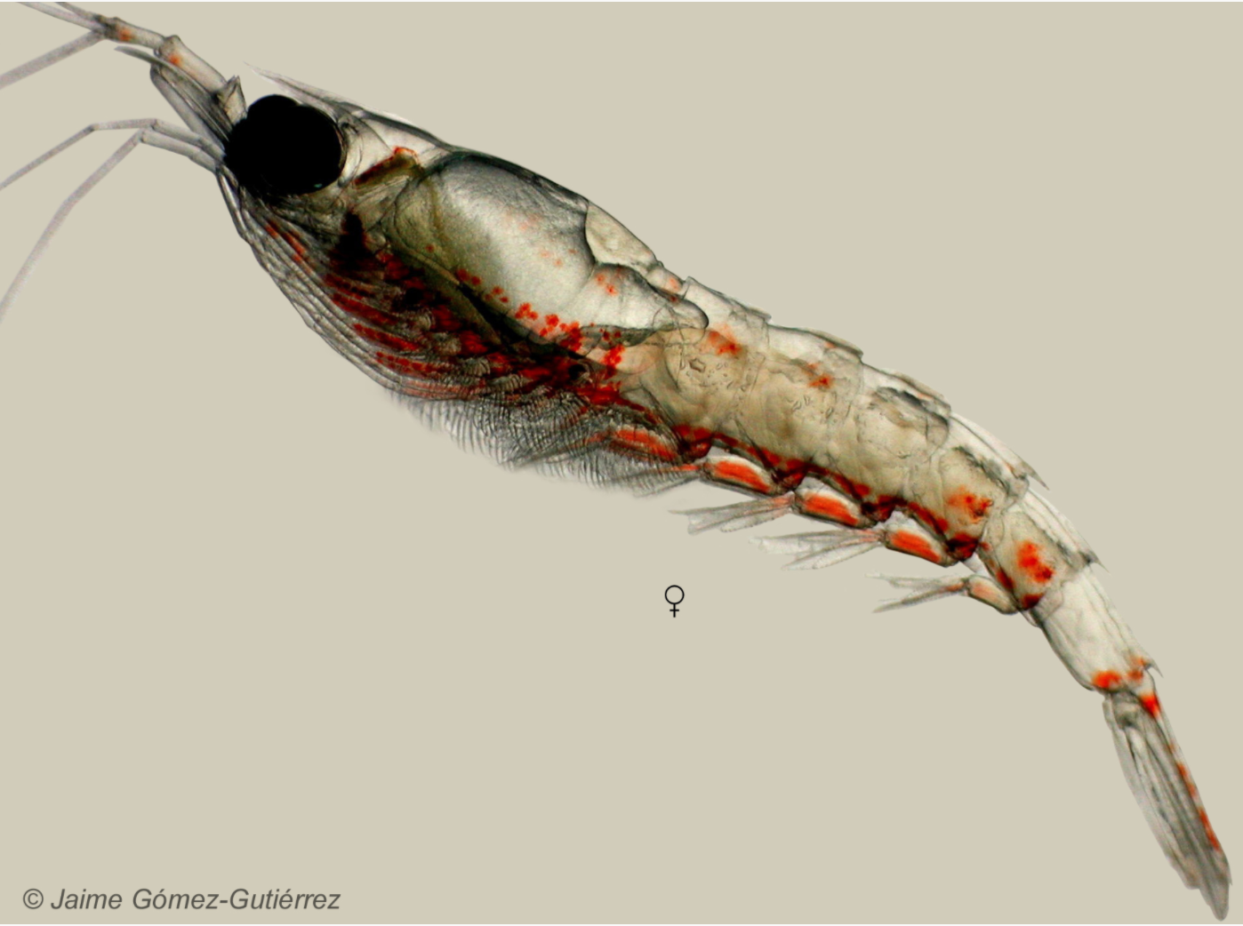
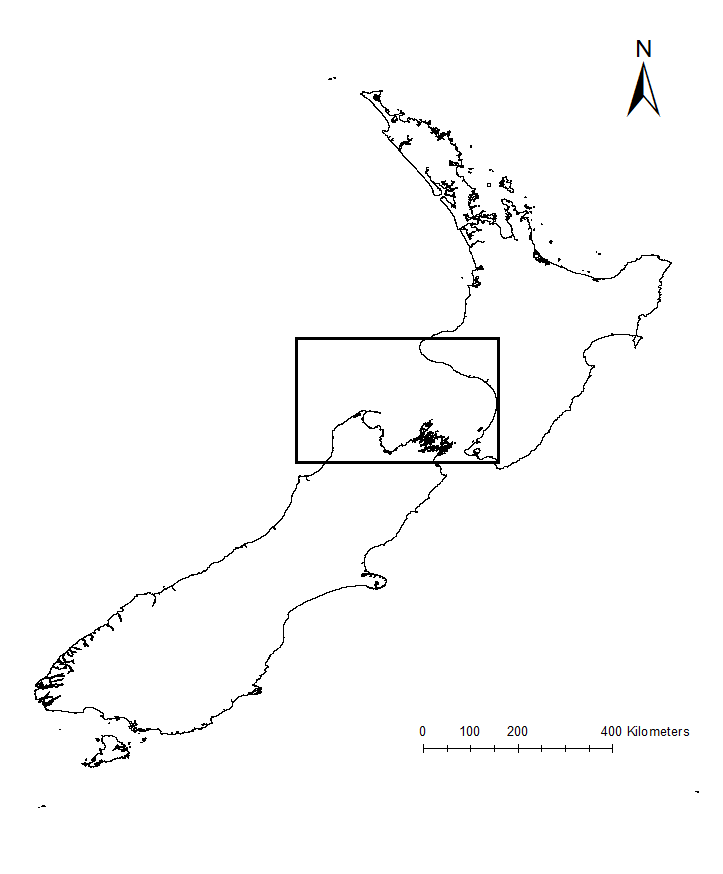
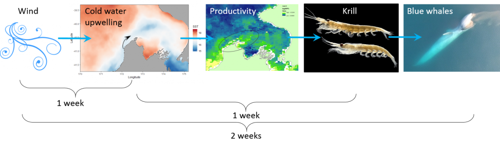
In the South Taranaki Bight (STB) region of New Zealand, where the GEMM lab has been studying blue whales for the past decade (Torres 2013), the New Zealand song type is recorded year-round (Barlow et al. 2018). New Zealand blue whales rely on a productive upwelling system in the STB that supports an important foraging ground (Barlow et al. 2020, 2021). Antarctic blue whales also seasonally pass through New Zealand waters, likely along their migratory pathway between polar feeding grounds and lower latitude areas (Warren et al. 2021). What does it mean in terms of population connectivity or separation when two different populations occasionally share the same waters? How do these different populations ecologically partition the space they occupy? What drives their differing occurrence patterns? These are the sorts of questions I am diving into as we continue to explore the depths of our acoustic recordings from the STB region. We still have a lot to learn about these blue whales, and there is a lot to be learned through listening.
References:
Balcazar NE, Tripovich JS, Klinck H, Nieukirk SL, Mellinger DK, Dziak RP, Rogers TL (2015) Calls reveal population structure of blue whales across the Southeast Indian Ocean and the Southwest Pacific Ocean. J Mammal 96:1184–1193.
Barlow DR, Bernard KS, Escobar-Flores P, Palacios DM, Torres LG (2020) Links in the trophic chain: Modeling functional relationships between in situ oceanography, krill, and blue whale distribution under different oceanographic regimes. Mar Ecol Prog Ser 642:207–225.
Barlow DR, Klinck H, Ponirakis D, Garvey C, Torres LG (2021) Temporal and spatial lags between wind, coastal upwelling, and blue whale occurrence. Sci Rep 11:1–10.
Barlow DR, Torres LG, Hodge KB, Steel D, Baker CS, Chandler TE, Bott N, Constantine R, Double MC, Gill P, Glasgow D, Hamner RM, Lilley C, Ogle M, Olson PA, Peters C, Stockin KA, Tessaglia-hymes CT, Klinck H (2018) Documentation of a New Zealand blue whale population based on multiple lines of evidence. Endanger Species Res 36:27–40.
Buchan SJ, Balcazar-Cabrera N, Stafford KM (2020) Seasonal acoustic presence of blue, fin, and minke whales off the Juan Fernández Archipelago, Chile (2007–2016). Mar Biodivers 50:1–10.
Leroy EC, Royer JY, Alling A, Maslen B, Rogers TL (2021) Multiple pygmy blue whale acoustic populations in the Indian Ocean: whale song identifies a possible new population. Sci Rep 11:8762.
Leroy EC, Samaran F, Stafford KM, Bonnel J, Royer JY (2018) Broad-scale study of the seasonal and geographic occurrence of blue and fin whales in the Southern Indian Ocean. Endanger Species Res 37:289–300.
Lewis LA, Calambokidis J, Stimpert AK, Fahlbusch J, Friedlaender AS, Mckenna MF, Mesnick SL, Oleson EM, Southall BL, Szesciorka AR, Širović A (2018) Context-dependent variability in blue whale acoustic behaviour. R Soc Open Sci 5.
McCauley RD, Gavrilov AN, Jolli CD, Ward R, Gill PC (2018) Pygmy blue and Antarctic blue whale presence , distribution and population parameters in southern Australia based on passive acoustics. Deep Res Part II 158:154–168.
McDonald MA, Mesnick SL, Hildebrand JA (2006) Biogeographic characterisation of blue whale song worldwide: using song to identify populations. J Cetacean Res Manag 8:55–65.
Oleson EM, Wiggins SM, Hildebrand JA (2007) Temporal separation of blue whale call types on a southern California feeding ground. Anim Behav 74:881–894.
Samaran F, Adam O, Guinet C (2010) Discovery of a mid-latitude sympatric area for two Southern Hemisphere blue whale subspecies. Endanger Species Res 12:157–165.
Samaran F, Stafford KM, Branch TA, Gedamke J, Royer J, Dziak RP, Guinet C (2013) Seasonal and Geographic Variation of Southern Blue Whale Subspecies in the Indian Ocean. PLoS One 8:e71561.
Torres LG (2013) Evidence for an unrecognised blue whale foraging ground in New Zealand. New Zeal J Mar Freshw Res 47:235–248.
Tripovich JS, Klinck H, Nieukirk SL, Adams T, Mellinger DK, Balcazar NE, Klinck K, Hall EJS, Rogers TL (2015) Temporal Segregation of the Australian and Antarctic Blue Whale Call Types (Balaenoptera musculus spp.). J Mammal 96:603–610.
Warren VE, Širović A, McPherson C, Goetz KT, Radford CA, Constantine R (2021) Passive Acoustic Monitoring Reveals Spatio-Temporal Distributions of Antarctic and Pygmy Blue Whales Around Central New Zealand. Front Mar Sci 7:1–14.