By Rachel Kaplan, PhD student, OSU College of Earth, Ocean and Atmospheric Sciences and Department of Fisheries, Wildlife, & Conservation Sciences, Geospatial Ecology of Marine Megafauna Lab
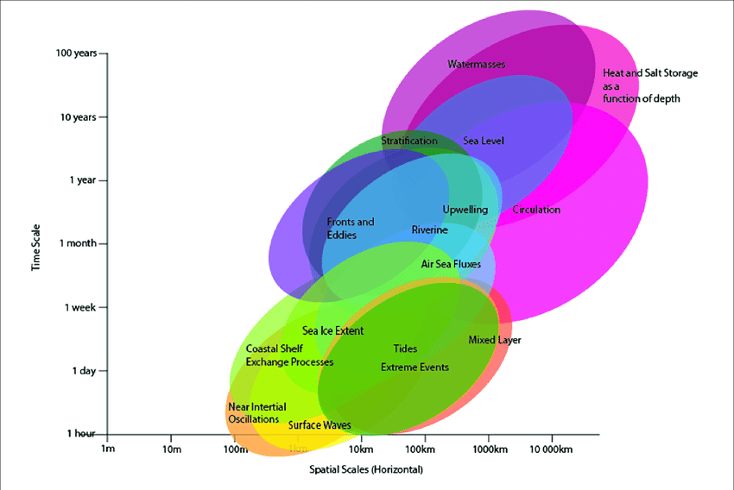
Ocean ecosystems are complex and dynamic, shaped by the interconnected physical and biogeochemical processes that operate across a variety of timescales. A trip on the “ocean conveyer belt”, which transports water from the North Atlantic across the global ocean and back in a process called thermohaline circulation, takes about a thousand years to complete. Phytoplankton blooms, which cycle nutrients through the surface ocean and feed marine animals, often occur at the crucial, food-poor moment of spring, and last for weeks or months. The entanglement of a whale in fishing gear, a major anthropogenic threat to ocean life that drives the GEMM Lab’s Project OPAL, can happen in seconds.
Compounding this complexity, even the timescales that research has clarified are changing. Many processes in the ocean are shifting – and often accelerating – due to global climate change. Images of melting sea ice, calving glaciers, and coastal erosion all exemplify our natural world’s rapid reorganization, and even discrete events can have dramatic repercussions and leave their mark for years. For example, a marine heatwave that occurred in 2014-2015 raised temperatures up to 2.5° C warmer than usual, redistributed species northward along the United States’ West Coast, spurred harmful algal blooms, and shut down fisheries. The toxic blooms also caused marine mammal strandings, domoic acid poisoning in California sea lions, and seabird mass death events (McCabe et al., 2016).
As humans seek to manage ocean ecosystems and mitigate the effects of climate change, our political processes have their own time scales, interconnected cycles, and stochasticity, just like the ocean. At the federal level in the United States, the legislative process takes place over months to decades, sometimes punctuated by relatively quicker actions enacted through Executive Orders. In addition, just as plankton have their turnover times, so do governmental branches. Both the legislative branch and the executive branch change frequently, with new members of Congress coming in every two years, and the president and administration changing every four or eight years. Turnover in both of these branches may constitute a total regime shift, with new members seeking to redirect science policy efforts.
The friction between oceanic and political timescales has historically made crafting effective ocean conservation policy difficult. In recent years, the policy approach of “adaptive management” has sought to respond to the challenges at the tricky intersection of politics, climate change, and ocean ecosystems. The U.S. Department of the Interior’s Technical Guide to Adaptive Management highlights its capacity to deal with the uncertainty inherent to changing ecosystems, and its ability to accommodate progress made through research: “Adaptive management [is a decision process that] promotes flexible decision making that can be adjusted in the face of uncertainties as outcomes from management actions and other events become better understood. Careful monitoring of these outcomes both advances scientific understanding and helps adjust policies or operations as part of an iterative learning process” (Williams et al, 2009).
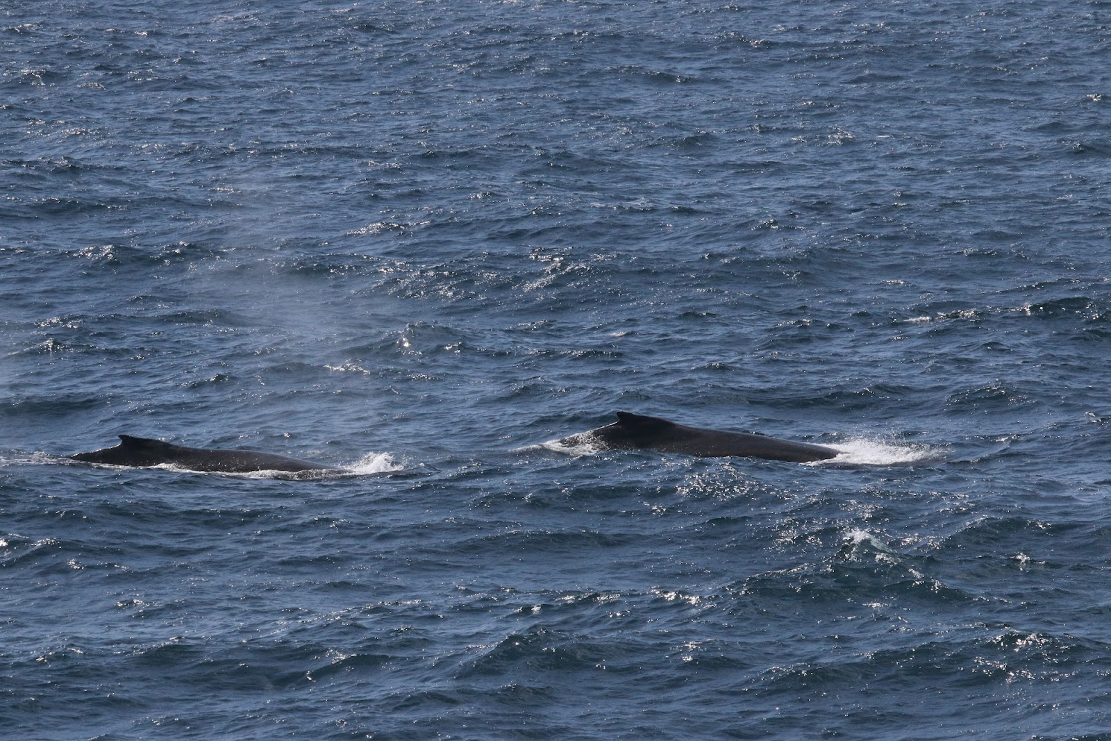
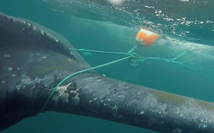
Over the last several years, adaptive management policy approaches have been key as resource managers along the West Coast have responded to the problem of whale entanglement in fishing gear. When the 2014-2015 marine heatwave event caused anomalously low krill abundance in the central California Current region, humpback whales used a tactic called “prey-switching”, and fed on inshore anchovy schools rather than offshore krill patches. The resulting habitat compression fueled an increase in humpback whale entanglement events in Dungeness crab fishing gear (Santora et al, 2020).
This sudden uptick in whale entanglements necessitated strategic management responses along the West Coast. In 2017, the California Dungeness Crab Fishing Gear Working Group developed the Risk Assessment and Mitigation Program (RAMP) to analyze real-time whale distribution and ocean condition data during the fishing season, and provide contemporaneous assessments of entanglement risk to the state’s Department of Fish and Wildlife. The Oregon Whale Entanglement Working Group (OWEWG) formed in 2017, tasked with developing options to reduce risk. Oregon Department of Fish and Wildlife (ODFW) has guided whale entanglement reduction efforts by identifying four areas of ongoing work: accountability, risk reduction, best management practices, and research – with regular, scheduled reviews of the regulations and opportunities to update and adjust them.
The need for research to support the best possible policy is where the GEMM Lab comes in. ODFW has established partnerships with Oregon State University and Oregon Sea Grant in order to improve understanding of whale distributions along the coast that can inform management efforts. Being involved in this cooperative “iterative learning process” is exactly why I’m so glad to be part of Project OPAL. Initial results from this work have already shaped ODFW’s regulations, and the framework of adaptive management and assessment means that regulations can continue being updated as we learn more through our research.
Ecosystem management will always be complex, just like ecosystems themselves. Today, the pace at which the climate is changing causes many people concern and even despair (Bryndum-Buchholz, 2022). Building adaptive approaches into marine policymaking, like the ones in use off the West Coast, introduces a new timescale into the U.S. policy cycle – one more in line with the rapid changes that are occurring within our dynamic ocean.
References
Williams, B. L., Szaro, R. C., and Shapiro, C. D. 2009. Adaptive management: the U.S. Department of the Interior Technical Guide. Adaptive Management Working Group, v pp.
Bryndum-Buchholz, A. (2022). Keeping up hope as an early career climate-impact scientist. ICES Journal of Marine Science, 79(9), 2345–2350. https://doi.org/10.1093/icesjms/fsac180
McCabe, R. M., Hickey, B. M., Kudela, R. M., Lefebvre, K. A., Adams, N. G., Bill, B. D., Gulland, F. M., Thomson, R. E., Cochlan, W. P., & Trainer, V. L. (2016). An unprecedented coastwide toxic algal bloom linked to anomalous ocean conditions. Geophys Res Lett, 43(19), 10366–10376. https://doi.org/10.1002/2016GL070023
Santora, J. A., Sydeman, W. J., Schroeder, I. D., Wells, B. K., & Field, J. C. (2011). Mesoscale structure and oceanographic determinants of krill hotspots in the California Current: Implications for trophic transfer and conservation. Progress in Oceanography, 91(4), 397–409. https://doi.org/10.1016/j.pocean.2011.04.002
Sloyan, B. M., Wilkin, J., Hill, K. L., Chidichimo, M. P., Cronin, M. F., Johannessen, J. A., Karstensen, J., Krug, M., Lee, T., Oka, E., Palmer, M. D., Rabe, B., Speich, S., von Schuckmann, K., Weller, R. A., & Yu, W. (2019). Evolving the Physical Global Ocean Observing System for Research and Application Services Through International Coordination. Frontiers in Marine Science, 6, 449. https://doi.org/10.3389/fmars.2019.00449