Significant others? Thinking beyond p-values in science

By Natalie Chazal, PhD student, OSU Department of Fisheries, Wildlife, & Conservation Sciences, Geospatial Ecology of Marine Megafauna Lab

Scientific inquiry relies on quantifying how certain we are of the differences we see in observations. This means that we must look at phenomena based on probabilities that we calculate from observed data, or data that we collect from sampling efforts. Historically, p-values have served as a relatively ubiquitous tool for assessing the strength of evidence in support of a hypothesis. However, as our understanding of statistical methods evolves, so does the scrutiny surrounding the appropriateness and interpretation of p-values. In the realm of research, the debate surrounding the use of p-values for determining statistical significance has sparked some controversy and reflection within the academic community. 

What is a p-value?

To understand the debate itself, we need to understand what a p-value is. The p-value represents the probability of obtaining a result as extreme as, or more extreme than, the observed data, under the assumption that there is no true difference or relationship between groups or variables. Traditionally, a p-value below a predetermined threshold (often 0.05) is considered statistically significant, suggesting that the observed data are unlikely (i.e., a 5% probability) to have occurred by chance alone. Many statistical tests provide p-values, which gives us a unified framework for interpretation across a range of analyses.

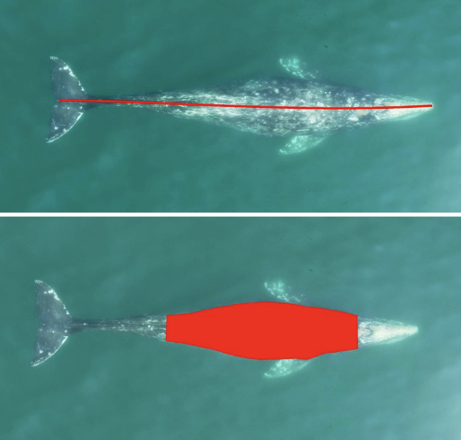
To illustrate this, imagine a study aimed at investigating the effects of underwater noise pollution on the foraging behavior of gray whales. Researchers collect data on the diving behavior of gray whales in both noisy and quiet regions of the ocean.

Drawings of gray whales with tags (depicted by orange shapes) in quiet areas (left) and noisy areas (right). 

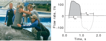
In this example, the researchers hypothesize that gray whales stop foraging and ultimately change their diving behavior in response to increased marine noise pollution. The data collected from this hypothetical scenario could come from tags equipped with sensors that record diving depth, duration, and location, allowing us to calculate the exact length of time spent foraging. Data would be collected from both noisy areas (maybe near shipping lanes or industrial sites) and quiet areas (more remote regions with minimal human activity). 

To assess the significance of the differences between the two noise regimes, researchers may use statistical tests like t-tests to compare two groups. In our example, researchers use a t-test to compare the average foraging time between whales in noisy and quiet regimes. The next step would be to define hypotheses about the differences we expect to see. The null hypothesis (HN) would be that there is no difference in the average foraging time (X) between noisy and quiet areas: 

Scenario where the noisy area does not elicit a behavioral response that can be detected by the data collected by the tags (orange shapes on whales back). The lower graph shows the distribution of the data (foraging time) for the noisy and the quiet areas. The means of this data (X) are not different. 

And the alternative hypothesis (HA) would be that there is a difference between the noisy and quiet areas: 

Scenario where the noisy area elicits a behavioral response (swimming more towards the surface instead of foraging) that can be detected by the data collected by the tags (orange shapes on whales back). The lower graph shows the distribution of the data (foraging time) for the noisy and the quiet areas. The means of this data (X) are different with the noisy mean foraging time (pink) being lower than the quiet mean foraging time (blue).

For now, we will skip over the nitty gritty of a t-test and just say that the researchers get a “t-score” that says whether or not there is a difference in the means (X) of the quiet and noisy areas. A larger t-score means that there is a difference in the means whereas a smaller t-score would indicate that the means are more similar. This t-score comes along with a p-value. Let’s say we get a t-score (green dot) that is associated with a p-value of 0.03 shown as the yellow area under the curve: 

The t-score is a test statistic that tells us how different the means of our observed data groups are from each other (green dot). The area under the t-distribution that is above the t-score is the p-value (yellow shaded area).

A p-value of 0.03 means that there is a 3% probability of obtaining these observed differences in foraging time between noisy and quiet areas purely by chance, which assumes that the null hypothesis is true (that there is no difference). We usually compare this p-value to a threshold value to say whether this finding is significant. We set this threshold before looking at the results of the test. If the threshold is above our value, like 0.05, then we can “reject the null hypothesis” and conclude that there is a significant difference in foraging time between noisy and quiet areas (green check mark scenario). On the flip-side, if the threshold that we set before our results is too low (0.01), then we will “fail to reject the null hypothesis” and conclude that there was no significant difference in foraging time between noisy and quiet areas (red check mark scenario). The reason that we don’t ever “accept the null” is because we are testing an alternative hypothesis with observations and if those observations are consistent with the null rather than the alternative, this is not evidence for the null because it could be consistent with a different alternative hypothesis that we are not yet testing for.

When our pre-set threshold to determine significance is above or greater than our p-value that was calculated we have enough evidence to ‘reject the null hypothesis’ (left figure) whereas if our p-value is lower or smaller than our calculated p-value, then we ‘fail to reject the null hypothesis’ (right figure).

In this example, the use of p-values helps the researchers quantify the strength of evidence for their hypothesis and determine whether the observed differences in gray whale behavior are likely to be meaningful or merely due to chance. 

The Debate

Despite its widespread use, the reliance on p-values has been met with criticism. Firstly, because p-values are so ubiquitous, it can be easy to calculate them with or without enough critical thinking or interpretation. This critical thinking should include an understanding of what is biologically relevant and avoid the trap of using binary language like significant or non-significant results instead of looking directly at the uncertainty of your results. One of the other most common misconceptions about p-values is that they can measure the direct probability of the null hypothesis being true. As amazing as that would be, in reality we can only use p-values to understand the probability of our observed data. Additionally, it’s common to conflate the significance or magnitude of the p-value with effect size (which is the strength of the relationship between the variables). You can have a small p-value for an effect that isn’t very large or meaningful, especially if you have a large sample size. Sample size is an important metric to report. Larger number of samples generally means more precise estimates, higher statistical power, increased generalizability, and higher possibility for replication.

Furthermore, in studies that require multiple comparisons (i.e. multiple statistical analyses are done in a single study), there is an increased likelihood of observing false positives because each test introduces a chance of obtaining a significant result by random variability alone. In p-value language, a “false positive” is when you say something is significant (below your p-value threshold) when it actually is not, and a “false negative” is when you say something is not significant (above the p-value threshold) when it actually is. So, in terms of multiple comparisons, if there are no adjustments made for the increased risk of false positives, this can potentially lead to inaccurate conclusions of significance.

In our example using foraging time in gray whales, we didn’t consider the context of our findings. To make this a more reliable study, we have to consider factors like the number of whales tagged (sample size!), the magnitude of noise near the tagged whales, other variables in the environment (e.g. prey availability) that could affect our results, and the ecological significance in the difference in foraging time that was found. To make robust conclusions, we need to carefully build hypotheses and study designs that will answer the questions we seek. We must then carefully choose the statistical tests that we use and explore how our data align with the assumptions that these tests make. It’s essential to contextualize our results within the bounds of our study design and broader ecological system. Finally, performing sensitivity analyses (e.g. running the same tests multiple times on slightly different datasets) ensures that our results are stable over a variety of different model parameters and assumptions. 

In the real world, there have been many studies done on the effects of noise pollution on baleen whale behavior that incorporate multiple sources of variance and bias to get robust results that show behavioral responses and physiological consequences to anthropogenic sound stressors (Melcón et al. 2012, Blair et al. 2016, Gailey et al. 2022, Lemos et al. 2022).

Moving Beyond P-values

There has been growing interest in reassessing the role of p-values in scientific inference and publishing. Scientists appreciate p-values because they provide one clear numeric threshold to determine significance of their results. However, the reality is more complicated than this binary approach. We have to explore the uncertainty around these estimates and test statistics (e.g. t-score) and what they represent ecologically. One avenue to explore might be focusing more on effect sizes and confidence intervals as more informative measures of the magnitude and precision of observed effects. There has also been a shift towards using Bayesian methods, which allow for the incorporation of prior knowledge and a more nuanced quantification of uncertainty.

Bayesian methods in particular are a leading alternative to p-values because instead of looking at how likely our observations are given a null hypothesis, we get a direct probability of the hypothesis given our data. For example, we can use Bayes factor for our noisy vs quiet gray whale behavioral t-test (Johnson et al. 2023). Bayes factor measures the likelihood of the data being observed for each hypothesis separately (instead of assuming the null hypothesis is true) so if we calculate a Bayes factor of 3 for the alternative hypothesis (HA), we could directly say that it is 3 times more likely for there to be decreased foraging time in a noisy area than for there to be no difference in the noisy vs quiet group. But that is just one example of Bayesian methods at work. The GEMM lab uses Bayesian methods in many projects from Lisa’s spatial capture-recapture models (link to blog) and Dawn’s blue whale abundance estimates (Barlow et al. 2018) to quantifying uncertainty associated with drone photogrammetry data collection methods in KC’s body size models (link to blog). 

Ultimately, the debate surrounding p-values highlights the necessity of nuanced and transparent approaches to statistical inference in scientific research. Rather than relying solely on arbitrary thresholds, researchers can consider the context, relevance, and robustness of their findings. From justifying our significance thresholds to directly describing parameters based on probability, we have increasingly powerful tools to improve the methodological rigor of our studies. 

References

Agathokleous, E., 2022. Environmental pollution impacts: Are p values over-valued? Science of The Total Environment 850, 157807. https://doi.org/10.1016/j.scitotenv.2022.157807

Barlow, D.R., Torres, L.G., Hodge, K.B., Steel, D., Baker, C.S., Chandler, T.E., Bott, N., Constantine, R., Double, M.C., Gill, P., Glasgow, D., Hamner, R.M., Lilley, C., Ogle, M., Olson, P.A., Peters, C., Stockin, K.A., Tessaglia-Hymes, C.T., Klinck, H., 2018. Documentation of a New Zealand blue whale population based on multiple lines of evidence. Endangered Species Research 36, 27–40. https://doi.org/10.3354/esr00891

Blair, H.B., Merchant, N.D., Friedlaender, A.S., Wiley, D.N., Parks, S.E., 2016. Evidence for ship noise impacts on humpback whale foraging behaviour. Biol Lett 12, 20160005. https://doi.org/10.1098/rsbl.2016.0005

Brophy, C., 2015. Should ecologists be banned from using p-values? Journal of Ecology Blog. URL https://jecologyblog.com/2015/03/06/should-ecologists-be-banned-from-using-p-values/ (accessed 4.19.24).

Castilho, L.B., Prado, P.I., 2021. Towards a pragmatic use of statistics in ecology. PeerJ 9, e12090. https://doi.org/10.7717/peerj.12090

Gailey, G., Sychenko, O., Zykov, M., Rutenko, A., Blanchard, A., Melton, R.H., 2022. Western gray whale behavioral response to seismic surveys during their foraging season. Environ Monit Assess 194, 740. https://doi.org/10.1007/s10661-022-10023-w

Halsey, L.G., 2019. The reign of the p-value is over: what alternative analyses could we employ to fill the power vacuum? Biology Letters 15, 20190174. https://doi.org/10.1098/rsbl.2019.0174

Johnson, V.E., Pramanik, S., Shudde, R., 2023. Bayes factor functions for reporting outcomes of hypothesis tests. Proceedings of the National Academy of Sciences 120, e2217331120. https://doi.org/10.1073/pnas.2217331120

Lemos, L.S., Haxel, J.H., Olsen, A., Burnett, J.D., Smith, A., Chandler, T.E., Nieukirk, S.L., Larson, S.E., Hunt, K.E., Torres, L.G., 2022. Effects of vessel traffic and ocean noise on gray whale stress hormones. Sci Rep 12, 18580. https://doi.org/10.1038/s41598-022-14510-5

LU, Y., BELITSKAYA-LEVY, I., 2015. The debate about p-values. Shanghai Arch Psychiatry 27, 381–385. https://doi.org/10.11919/j.issn.1002-0829.216027

Melcón, M.L., Cummins, A.J., Kerosky, S.M., Roche, L.K., Wiggins, S.M., Hildebrand, J.A., 2012. Blue Whales Respond to Anthropogenic Noise. PLOS ONE 7, e32681. https://doi.org/10.1371/journal.pone.0032681

Murtaugh, P.A., 2014. In defense of P values. Ecology 95, 611–617. https://doi.org/10.1890/13-0590.1

Vidgen, B., Yasseri, T., 2016. P-Values: Misunderstood and Misused. Front. Phys. 4. https://doi.org/10.3389/fphy.2016.00006

Baleen analyses reveals patterns in foraging ecology and stress physiology in gray whales prior to death.

Dr. Alejandro A. Fernández Ajó, Postdoctoral Scholar, Marine Mammal Institute – OSU Department of Fisheries, Wildlife, & Conservation Sciences, Geospatial Ecology of Marine Megafauna (GEMM) Lab.

The Eastern North Pacific (ENP) gray whale population has experienced at least two recorded Unusual Mortality Events (UMEs), from 1999–2000 and from 2019 to 2024, during which many gray whales stranded along the Pacific coast from northern Mexico to the Alaskan Arctic, USA (Martínez-Aguilar et al., 2019; Urbán, 2020). Several factors have been considered as possible causes for the high number of gray whale’s strandings, including variation in Arctic prey availability and the duration of their feeding season caused by the timing of sea ice formation and breakup (Stewart et al., 2023), starvation, anthropogenically derived toxicants, biotoxins, infectious diseases, parasites, fisheries interactions, and ship strikes (F. Gulland et al., 2005). In the most recent UME, many of the stranded whales showed signs of emaciation, indicating malnutrition as a causal factor of death (Christiansen et al., 2021; Torres et al., 2022). While the poor condition of many of the stranded whales supports the idea of starvation as a cause for these mortalities, the underlying causes of malnutrition are unknown, and it is also unclear whether the whales’ decline in body condition was rapid or gradual.

Figure 1. Gray whale with baleen exposed. Photo: GEMM Lab  NOAA/NMFS permit #16111.

Large whales face a multitude of stressors in their environment, ranging from ocean noise to contaminants, climate change, and prey shifts. Understanding how individual whales respond to these disturbances is crucial for assessing potential impacts on the population as a whole. However, monitoring the health parameters and vital rates of whales presents significant challenges due to their large size, mobility, and the vast ranges of their marine habitat. Studying stranded whales can provide valuable insights into health risks, disease susceptibility, and the impacts of pollutants and other stressors on whale populations, thus informing conservation strategies (see post). Nonetheless, the quality of information obtained from necropsies heavily relies on the timeliness of stranding reports, as decomposition begins immediately after death, limiting detailed investigations into the cause of death. Therefore, establishing a robust network capable of promptly reporting and addressing stranding events is essential (Gulland & Stockin, 2020). An effective network involves having well-trained staff, proper infrastructure, sufficient funding, and the expertise and tools necessary to gather and analyze data and samples to infer their health and causes of mortality.

During my doctoral dissertation, I worked to develop and ground truth the endocrine analyses of whale baleen as a novel sample type that can be used for retrospective assessments of the whale’s physiology (see my previous post & post). Baleen, the filter-feeding apparatus of mysticetes whales (Figure 1), consists of long fringed plates of keratinized tissue that grow continuously and slowly downward from the whale’s upper jaw. These plates are routinely collected at necropsies; and unlike other tissue types, they are durable and have minimum storage requirements; they can be preserved dry at room temperature, allowing for the analysis of both historical and current whale populations. Moreover, while most sample types used for studying whale health and physiology provide a single time-point measure of current circulating hormone levels (e.g., skin or respiratory vapor) or hold integrated information from the previous few hours or days (e.g., urine and feces), baleen tissue provides a unique opportunity for retrospective and longitudinal analyses of multiple biological parameters of the individual during the time that the tissue was grown, i.e., months to years prior to death, helping to describe the whale’s physiology, migration patterns, and exposure to pollutants (see my previous post).

In our recent study, “A longitudinal study of endocrinology and foraging ecology of subadult gray whales prior to death based on baleen analysis”, published in the journal General and Comparative Endocrinology, we examine isotope and hormone levels in the baleen of five young gray whales stranded in central Oregon during the most recent UME. Our primary objectives were to retrospectively examine the hormone and isotopic profiles of the individual whales prior to mortality, assess potential factors contributing to death, and identify the timing for the onset of chronic illness leading to mortality. Our analysis included tracing longitudinal changes in (1) stable isotope values in baleen (δ13C and δ15N), which allowed us to infer the baleen growth rate and assess the seasonal changes in diet and foraging location in large whales (Figure 2), along with the quantification of (2) two adrenal glucocorticoid steroids that are biomarkers for the whale’s stress response, (3) one thyroid hormone (triiodothyronine, T3) as an indicator of nutritional state, and (4) two sex hormones, progesterone and testosterone, to infer about reproductive status and sexual maturity. By integrating isotopic and hormonal methodologies, our study demonstrates how baleen analysis offers a comprehensive narrative of the endocrine and trophic ecology of individual whales over time.

Figure 2. Gray whales, like other large marine mammals that rely on built-up energy reserves, exhibit distinct seasonal shifts in their feeding habits. During summer, these whales feed at the ocean’s bottom, consuming organisms lower in the food chain, which is reflected in lower nitrogen values in their baleen (summer foraging). In winter, however, they must rely on their own fat reserves, causing an increase in nitrogen values (wintering). In this plot we can observe the oscillations in δ15N over time; this information allows us to estimate the baleen growth rate. Our results suggest that gray whale baleen holds a record of around 1.3 years of stable isotopes and hormone data prior to the time of death (Fernandez Ajo et al. 2024). The red cross in the X-axis, indicate the time of death. Gray whale illustration https://www.fisheries.noaa.gov/species/gray-whale

Our endocrine assessments revealed detailed profiles of stress-related hormones (glucocorticoids, cortisol) and thyroid hormones along the lengths of the baleen. We found increased levels of cortisol in whales that died from unknown causes, starting about eight months prior to their deaths. This suggests these whales were under prolonged stress before dying. In contrast, in the case of a whale killed acutely by a killer whale, cortisol levels were low and constant prior to death, indicating this individual was likely in good health prior to the sudden attack. In terms of thyroid activity, indicated by T3 hormone levels, we found a gradual increase over several months in the whales that died of unknown causes. This pattern is not typically expected, as stress usually suppresses thyroid function. This anomaly could suggest an adaptive response to maintain body temperature and metabolism in potentially malnourished whales. Regarding the sex hormones, as expected for this age class, we found no significant fluctuations or spikes that would indicate sexual maturity in these young whales (Figure 3).

Figure 3. Longitudinal hormone profiles in an individual gray whale that died due to unknown causes (left) and one that died acutely due to orca predation (right). Note the pronounced elevations in cortisol levels (indicative of stress) and T3 prior to death in the case of unknown cause of death, while hormone levels remained low and constant prior to death in the whale acutely killed. Sex hormones do not present any clear oscillations, indicating that these whales were likely sexually immature. The red cross in the X-axis, indicate the time of death. Killer whale (Orcinus orca) illustration https://www.fisheries.noaa.gov/species/ killer-whale

Although commercial whaling is currently banned and several whale populations show evidence of recovery, today’s whales are exposed to a variety of other human stressors that cause significant lethal and non-lethal impacts (e.g., entanglement in fishing gear, vessel strikes, shipping noise, climate change, etc.; reviewed in Thomas et al., 2016). The recovery and conservation of large whale populations is particularly important to the oceanic environment due to their key ecological role and unique biological traits (See my previous post). Our research demonstrates the strengths of using baleen as a tool for the retrospective assessments of whale endocrinology and trophic ecology. As the Eastern North Pacific gray whale population faces recurring challenges, indicated by fluctuating numbers and unusual mortality events, innovative techniques like the baleen analysis presented here, are essential to investigate the causes of mortality and inform management, helping us understand not only the immediate causes of death but also broader environmental and ecological changes affecting their survival. Broadly implementing this approach with a greater sample size of baleen collected across a larger spatial and temporal range could significantly improve our strategies for conservation and management of baleen whales.

Did you enjoy this blog? Want to learn more about marine life, research, and
conservation? Subscribe to our blog and get a weekly message when we post a new
blog. Just add your name and email into the subscribe box below.

Loading

References

Christiansen, F., Rodríguez-González, F., Martínez-Aguilar, S., Urbán, J., Swartz, S., Warick, H., Vivier, F., & Bejder, L. (2021). Poor body condition associated with an unusual mortality event in gray whales. Marine Ecology Progress Series, 658, 237–252. https://doi.org/10.3354/meps13585

Gulland, F. M. D., & Stockin, K. A. (2020). Harmonizing global strandings response. European Cetacean Society Special Publication Series.

Gulland, F., Pérez-Cortés, H., Urbán, J. R., Rojas-Bracho, L., Ylitalo, G., Weir, J., Norman, S., Muto, M., Rugh, D., Kreuder, C., & Rowles, T. (2005). Eastern North Pacific gray whale (Eschrichtius robustus) unusual mortality event, 1999-2000. U.S. Department of Commerce. NOAA Technical Memorandum. NMFS-AFSC-150., March, 33 pp. http://www.afsc.noaa.gov/publications/AFSC-TM/NOAA-TM-AFSC-150.pdf

Martínez-Aguilar, S., Mariano-Meléndez, E., López-Paz, N., Castillo-Romero, F., Zaragoza-aguilar, G. A., Rivera-Rodriguez, J., Zaragoza-Aguilar, A., Swartz, S., Viloria-Gómora, L., & Urbán, J. R. (2019). Gray whale (Eschrichtius robustus) stranding records in Mexico during the winter breeding season in 2019. Report of the International Whaling Commission. Document SC/68A/CMP/14, May.

Stewart, J. D., Joyce, T. W., Durban, J. W., Calambokidis, J., Fauquier, D., Fearnbach, H., Grebmeier, J. M., Lynn, M., Manizza, M., Perryman, W. L., Tinker, M. T., & Weller, D. W. (2023). Boom-bust cycles in gray whales associated with dynamic and changing Arctic conditions. Science, 382(6667), 207–211. https://doi.org/10.1126/science.adi1847

Torres, L. G., Bird, C. N., Rodríguez-González, F., Christiansen, F., Bejder, L., Lemos, L., Urban R, J., Swartz, S., Willoughby, A., Hewitt, J., & Bierlich, KC. (2022). Range-Wide Comparison of Gray Whale Body Condition Reveals Contrasting Sub-Population Health Characteristics and Vulnerability to Environmental Change. Frontiers in Marine Science, 9. https://doi.org/10.3389/fmars.2022.867258

Urbán, R. (2020). Gray whale stranding records in Mexico during the 2020 winter breeding season. Unpublished Paper SC/68B/CMP/13 Presented to the IWC Scientific Committee, Cambridge.

A MOSAIC of species, datasets, tools, and collaborators

By Dr. Dawn Barlow, Postdoctoral Scholar, OSU Department of Fisheries, Wildlife, and Conservation Sciences, Geospatial Ecology of Marine Megafauna Lab

Imagine you are 50 nautical miles from shore, perched on the observation platform of a research vessel. The ocean is blue, calm, and seems—for all intents and purposes—empty. No birds fly overhead, nothing disturbs the rolling swells except the occasional whitecap from a light breeze. The view through your binoculars is excellent, and in the distance, you spot a disturbance at the surface of the water. As the ship gets closer, you see splashing, and a flurry of activity emerges as a large group of dolphins leap and dive, likely chasing a school of fish. They swim along with the ship, riding the bow-wave in a brief break from their activity. Birds circle in the air above them and float on the water around them. Together with your team of observers, you rush to record the species, the number of animals, their distance to the ship, and their behavior. The research vessel carries along its pre-determined trackline, and the feeding frenzy of birds and dolphins fades off behind you as quickly as it came. You return to scanning the blue water.

Craig Hayslip and Dawn Barlow scan for marine mammals from the crow’s nest (elevated observation platform) of the R/V Pacific Storm.

The marine environment is highly dynamic, and resources in the ocean are notoriously patchy. One of our main objectives in marine ecology is to understand what drives these ephemeral hotspots of species diversity and biological activity. This objective is particularly important now as the oceans warm and shift. In the context of rapid global climate change, there is a push to establish alternatives to fossil fuels that can support society’s energy needs while minimizing the carbon emissions that are a root cause of climate change. One emergent option is offshore wind, which has become a hot topic on the West Coast of the United States in recent years. The technology has the potential to supply a clean energy source, but the infrastructure could have environmental and societal impacts of its own, depending on where it is placed, how it is implemented, and when it is operational.

Northern right whale dolphins leap into the air. Photo by Craig Hayslip.

Any development in the marine environment, including alternative energy such as offshore wind, should be undertaken using the best available scientific knowledge of the ecosystem where it will be implemented. The Marine Mammal Institute’s collaborative project, Marine Offshore Species Assessments to Inform Clean energy (MOSAIC), was designed for just this reason. As the name “MOSAIC” implies, it is all about using different tools to compile different datasets to establish crucial baseline information on where marine mammals and seabirds are distributed in Oregon and Northern California, a region of interest for wind energy development.

A MOSAIC of species

The waters of Oregon and Northern California are rich with life. Numerous cetaceans are found here, from the largest species to ever live, the blue whale, to one of the smallest cetaceans, the harbor porpoise, with many species filling in the size range in between: fin whales, humpback whales, sperm whales, killer whales, Risso’s dolphins, Pacific white-sided dolphins, northern right whale dolphins, and Dall’s porpoises, to name a few. Seabirds likewise rely on these productive waters, from the large, graceful albatrosses that feature in maritime legends, to charismatic tufted puffins, to the little Leach’s storm petrels that could fit in the palm of your hand yet cover vast distances at sea. From our data collection efforts so far, we have already documented 16 cetacean species and 64 seabird species.

A Laysan albatross glides over the water’s surface. Photo by Will Kennerley.

A MOSAIC of data and tools

Schematic of the different components of the MOSAIC project. Graphic created by Solene Derville.

Through the four-year MOSAIC project, we are undertaking two years of visual surveys and passive acoustic monitoring from Cape Mendocino to the mouth of the Columbia River on the border of Oregon and Washington and seaward to the continental slope. Six comprehensive surveys for cetaceans and seabirds are being conducted aboard the R/V Pacific Storm following a carefully chosen trackline to cover a variety of habitats, including areas of interest to wind energy developers.

These dedicated surveys are complemented by additional surveys conducted aboard NOAA research vessels during collaborative expeditions in the Northern California Current, and ongoing aerial surveys in partnership with the United States Coast Guard through the GEMM Lab’s OPAL project. Three bottom-mounted hydrophones were deployed in August 2022, and are recording cetacean vocalizations and the ambient soundscape, and these recordings will be complemented by acoustic data that is being collected continuously by the Oceans Observing Initiative. In addition to these methods to collect broad-scale species distribution information, concurrent efforts are being conducted via small boats to collect individual identification photographs of baleen whales and tissue biopsy samples for genetic analysis. Building on the legacy of satellite tracking here at the Marine Mammal Institute, the MOSAIC project is breathing new life into tag data from large whales to assess movement patterns over many years and determine the amount of time spent within our study area.

A curious fin whale approaches the R/V Pacific Storm during one of the visual surveys. Photo by Craig Hayslip.
Survey tracklines extending between the Columbia River and Cape Mendocino, designed for the MOSAIC visual surveys aboard the R/V Pacific Storm.

The resulting species occurrence data from visual surveys and acoustic monitoring will be integrated to develop Species Distribution Models for the many different species in our study region. Identification photographs of individual baleen whales, DNA profiles from whale biopsy samples, and data from satellite-tagged whales will provide detailed insight into whale population structure, behavior, and site fidelity (i.e., how long they typically stay in a given area), which will add important context to the distribution data we collect through the visual surveys and acoustic monitoring. The models will be implemented to produce maps of predicted species occurrence patterns, describing when and where we expect different cetaceans and seabirds to be under different environmental conditions.

With five visual surveys down, the MOSAIC team is gearing up for one final survey this month. The hydrophones will be retrieved this summer. Then, with data in-hand, the team will dive deep into analysis.

A MOSAIC of collaborators

The MOSAIC-4 team waves from the crow’s nest (observation platform) of the R/V Pacific Storm. Photo by Craig Hayslip.

The collaborative MOSAIC team brings together a diverse set of tools. The depth of expertise here at the Marine Mammal Institute spans a broad range of disciplines, well-positioned to provide robust scientific knowledge needed to inform alternative energy development in Oregon and Northern California waters.  

I have had the pleasure of participating in three of the six surveys aboard the R/V Pacific Storm, including leading one as Chief Scientist, and have collected visual survey data aboard NOAA Ship Bell M. Shimada and from United States Coast Guard helicopters over the years that will be incorporated in the MOSAIC of datasets for the project. This ecosystem is one that I feel deeply connected to from time spent in the field. Now, I am thrilled to dive into the analysis, and will lead the modeling of the visual survey data and the integration of the different components to produce species distribution maps for cetaceans and seabirds our study region.

This project is funded by the United States Department of Energy. The Principal Investigator is the Institute’s Director Dr. Lisa Ballance, and Co-Principal Investigators include Scott Baker, Barbara Lagerquist, Rachael Orben, Daniel Palacios, Kate Stafford, and Leigh Torres of the Marine Mammal Institute; John Calambokidis of the Cascadia Research Collective; and Elizabeth Becker of ManTech International Corp. For more information, please visit the project website, and stay tuned for updates as we enter the analysis phase.

Did you enjoy this blog? Want to learn more about marine life, research, and conservation? Subscribe to our blog and get a weekly alert when we make a new post! Just add your name into the subscribe box below!

Loading

An ‘X’travaganza! Introducing the Marine Mammal Institute’s Center of Drone Excellence (CODEX)

Dr. KC Bierlich, Postdoctoral Scholar, OSU Department of Fisheries, Wildlife, & Conservation Sciences, Geospatial Ecology of Marine Megafauna Lab

Drones are becoming more and more prevalent in marine mammal research, particularly for non-invasively obtaining morphological measurements of cetaceans via photogrammetry to identify important health metrics (see this and this previous blog). For example, the GEMM Lab uses drones for the GRANITE Project to study Pacific Coast Feeding Group (PCFG) gray whales and we have found that PCFG whales are skinnier and morphologically shorter with smaller skulls and flukes compared to the larger Eastern North Pacific (ENP) population. The GEMM Lab has also used drones to document variation in body condition across years and within a season, to diagnose pregnancy, and even measure blowholes.

While drone-based photogrammetry can provide major insight into cetacean ecology, several drone systems and protocols are used across the scientific community in these efforts, and no consistent method or centralized framework is established for quantifying and incorporating measurement uncertainty associated with these different drones. This lack of standardization restricts comparability across datasets, thus hindering our ability to effectively monitor populations and understand the drivers of variation (e.g., pollution, climate change, injury, noise).

We are excited to announce the Marine Mammal Institute’s (MMI) Center of Drone Excellence (CODEX), which focuses on developing analytical methods for using drones to non-invasively monitor marine mammal populations. CODEX is led by GEMM Lab member’s KC Bierlich, Leigh Torres, and Clara Bird and consists of other team members within and outside OSU. We draw from many years of trials, errors, headaches, and effort working with drones to study cetacean ecology in a variety of habitats and conditions on many different species.

Already CODEX has developed several open-source hardware and software tools. We developed, produced, and published LidarBoX (Bierlich et al., 2023), which is a 3D printed enclosure for a LiDAR altimeter system that can be easily attached and swapped between commercially available drones (i.e., DJI Inspire, DJI Mavic, and DJI Phantom) (Figure 1). Having a LidarBoX installed helps researchers obtain altitude readings with greater accuracy, yielding morphological measurements with less uncertainty. Since we developed LidarBoX, we have received over 35 orders to build this unit for other labs in national and international universities.

Figure 1. A ‘LidarBoX’ attached to a DJI Inspire 2. The LidarBoX is a 3D printed enclosure containing a LiDAR altimeter to help obtain more accurate altitude readings.

Additionally, CODEX recently released MorphoMetriX version 2 (v2), an easy-to-use photogrammetry software that provides users with the flexibility to obtain custom morphological measurements of megafauna in imagery with no knowledge of any scripting language (Torres and Bierlich, 2020). CollatriX is a user-friendly software for collating multiple MorphoMetriX outputs into a single dataframe and linking important metadata to photogrammetric measurements, such as altitude measured with a LidarBoX (Bird and Bierlich, 2020). CollatriX also automatically calculates several body condition metrics based on measurements from MorphoMetriX v2. CollatriX v2 is currently in beta-testing and scheduled to be released late Spring 2024. 

Figure 2. An example of a Pygmy blue whale imported into MorphoMetriX v2, open-source photogrammetry software. 

CODEX also recently developed two automated tools to help speed up the laborious manual processing of drone videos for obtaining morphological measurements (Bierlich & Karki et al., in revision). DeteX is a graphical user interface (GUI) that uses a deep learning model for automated detection of cetaceans in drone-based videos. Researchers can input their drone-based videos and DeteX will output frames containing whales at the surface. Users can then select which frames they want to use for measuring individual whales and then input these selected frames into XtraX, which is a GUI that uses a deep learning model to automatically extract body length and body condition measurements of cetaceans (Figure 4). We found automated measurements from XtraX to be similar (within 5%) of manual measurements. Importantly, using DeteX and XtraX takes about 10% of the time it would take to manually process the same videos, demonstrating how these tools greatly speed up obtaining key morphological data while maintaining accuracy, which is critical for effectively monitoring population health.

Figure 3. An example of an automated body length (top) and body condition (bottom) measurement of a gray whale using XtraX (Bierlich & Karki et al., in revision).

CODEX is also in the process of developing Xcertainty, an R package that uses a Bayesian statistical model to quantify and incorporate uncertainty associated with measurements from different drones (see this blog). Xcertainty is based on the Bayesian statistical model developed by Bierlich et al., (2021b; 2021a), which has been utilized by many studies with several different drones to compare body condition and body morphology across individuals and populations  (Bierlich et al., 2022; Torres et al., 2022; Barlow et al., 2023). Rather than a single point-estimate of a length measurement for an individual, Xcertainty produces a distribution of length measurements for an individual so that the length of a whale can be described by the mean of this distribution, and its uncertainty as the the variance or an interval around the mean (Figure 4). These outputs ensure measurements are robust and comparable across different drones because they provide a measure of the uncertainty around each measurement. For instance, a measurement with more uncertainty will have a wider distribution. The uncertainty associated with each measurement can be incorporated into analyses, which is key when detecting important differences or changes in individuals or populations, such as changes in body condition (blog).

Figure 4. An example of a posterior predictive distribution for total length of an individual blue whale produced by the ‘Xcertainty’ R package. The black bars represent the uncertainty around the mean value (the black dot) – the longer black bars represent the 95% highest posterior density (HPD) interval, and the shorter black bars represent the 65% HPD interval. 

CODEX has integrated all these lessons learned, open-source tools, and analytical approaches into a single framework of suggested best practices to help researchers enhance the quality, speed, and accuracy of obtaining important morphological measurements to manage vulnerable populations. These tools and frameworks are designed to be accommodating and accessible to researchers on various budgets and to facilitate cross-lab collaborations. CODEX plans to host workshops to educate and train researchers using drones on how to apply these tools within this framework within their own research practices. Potential future directions for CODEX include developing a system for using drones to drop suction-cup tags on whales and to collect thermal imagery of whales for health assessments. Stay up to date with all the CODEX ‘X’travaganza here: https://mmi.oregonstate.edu/centers-excellence/codex.  

Huge shout out to Suzie Winquist for designing the artwork for CODEX!

References

Barlow, D.R., Bierlich, K.C., Oestreich, W.K., Chiang, G., Durban, J.W., Goldbogen, J.A., Johnston, D.W., Leslie, M.S., Moore, M.J., Ryan, J.P. and Torres, L.G., 2023. Shaped by Their Environment: Variation in Blue Whale Morphology across Three Productive Coastal Ecosystems. Integrative Organismal Biology, [online] 5(1). https://doi.org/10.1093/iob/obad039.

Bierlich, K., Karki, S., Bird, C.N., Fern, A. and Torres, L.G., n.d. Automated body length and condition measurements of whales from drone videos for rapid assessment of population health. Marine Mammal Science.

Bierlich, K.C., Hewitt, J., Bird, C.N., Schick, R.S., Friedlaender, A., Torres, L.G., Dale, J., Goldbogen, J., Read, A.J., Calambokidis, J. and Johnston, D.W., 2021a. Comparing Uncertainty Associated With 1-, 2-, and 3D Aerial Photogrammetry-Based Body Condition Measurements of Baleen Whales. Frontiers in Marine Science, 8. https://doi.org/10.3389/fmars.2021.749943.

Bierlich, K.C., Hewitt, J., Schick, R.S., Pallin, L., Dale, J., Friedlaender, A.S., Christiansen, F., Sprogis, K.R., Dawn, A.H., Bird, C.N., Larsen, G.D., Nichols, R., Shero, M.R., Goldbogen, J., Read, A.J. and Johnston, D.W., 2022. Seasonal gain in body condition of foraging humpback whales along the Western Antarctic Peninsula. Frontiers in Marine Science, 9(1036860), pp.1–16. https://doi.org/10.3389/fmars.2022.1036860.

Bierlich, K.C., Schick, R.S., Hewitt, J., Dale, J., Goldbogen, J.A., Friedlaender, A.S. and Johnston, D.W., 2021b. Bayesian approach for predicting photogrammetric uncertainty in morphometric measurements derived from drones. Marine Ecology Progress Series, 673, pp.193–210. https://doi.org/10.3354/meps13814.

Bird, C. and Bierlich, K.C., 2020. CollatriX: A GUI to collate MorphoMetriX outputs. Journal of Open Source Software, 5(51), pp.2323–2328. https://doi.org/10.21105/joss.02328.

Torres, L.G., Bird, C.N., Rodríguez-González, F., Christiansen, F., Bejder, L., Lemos, L., Urban R, J., Swartz, S., Willoughby, A., Hewitt, J. and Bierlich, K.C., 2022. Range-Wide Comparison of Gray Whale Body Condition Reveals Contrasting Sub-Population Health Characteristics and Vulnerability to Environmental Change. Frontiers in Marine Science, 9(April), pp.1–13. https://doi.org/10.3389/fmars.2022.867258.

Torres, W. and Bierlich, K.C., 2020. MorphoMetriX: a photogrammetric measurement GUI for morphometric analysis of megafauna. Journal of Open Source Software, 5(45), pp.1825–1826. https://doi.org/10.21105/joss.01825.

Every breath [a whale] takes: How and why we study cetacean respiration

Clara Bird, PhD Candidate, OSU Department of Fisheries, Wildlife, and Conservation Sciences, Geospatial Ecology of Marine Megafauna Lab

We need energy to function and survive. For animals in the wild who may have limited food availability, knowing how they spend their energy is a critical question for many scientists because it fundamentally informs how we understand their decisions about where they go and what they do. The entire field of foraging theory is founded on the concept that animals optimize their ratio of energy in and energy out so that they have enough energy to survive, reproduce (pass on their genes), watch out for threats, if need be, and rest. And, if we understand an animal’s ‘typical’ energy budget, we can then try to predict how disturbance or environmental change will affect their actual energy budgets as a consequence of that change. But how do we measure energy expenditure?

The most commonly measured energy currency is oxygen. Since our cells use oxygen to produce energy (this is why we need oxygen to live), we can measure oxygen consumption as a metric of energy expenditure. The more oxygen we consume, the more energy we’re expending. In ideal lab settings, oxygen consumption can be accurately measured by placing the subject in a chamber where the oxygen flow can be controlled (Speakman, 1999). However, you can probably see how that approach is problematic for measuring oxygen consumption in most large free-living animals, especially cetaceans. It isn’t exactly feasible to put a whale in a box.

Image 1. A great tit in a metabolic chamber. Figure 1 from Broggi et al., 2009

Fortunately, a tool called a spirometer was developed to measure oxygen consumption in restrained cetaceans. A spirometer is a device that can be placed over the blowhole(s) of an individual to accurately measure the amount of air that is exhaled and inhaled (Figure 1).  For trained cetaceans in captivity (e.g., dolphins), spirometers can be used to quantify how respiration changes after the animal performs certain behaviors (Fahlman et al., 2019). The breathing patterns of diving mammals are particularly interesting because they cannot breathe during most of their exercise (energy expenditure) as they are underwater. So, their breathing patterns after a dive tell us a lot about how much energy they spent during that dive. For example, Fahlman et al. (2019) used spirometer data from dolphins in captivity to study how their breathing patterns changed while recovering from dives of different durations. Interestingly, they found that after longer dives, dolphins took larger breaths (i.e., inhaled more air) while recovering but did not change the number of breaths. This finding is particularly relevant to the work we are conducting in the GEMM lab, where we utilize breathing patterns to quantify the energy expenditure of cetaceans in the wild, where spirometers cannot be used.

Figure 1. Figure 1 from Sumich et al. (2023). Left: a spirometer being held over the blow holes of JJ, a gray whale calf at sea world in 1997; one of the rare times that a large baleen whale was in captivity and available for these measurements. Right: example of a plot created using the data from a spirometer over JJ’s blow holes. The duration of a “blow” (exhale followed by immediate inhale) is on the x-axis, the flow rate (in liters per second) is on the y-axis. The positive curve during the exhale shows that the whale strongly exhales a lot of air very quickly, then the negative curve shows the whale inhaling a lot of air very quickly.

In a previous blog, I described how inter-breath intervals (the time between consecutive blows) are useful for estimating energy expenditure in free-living cetaceans. Essentially, a shorter interval indicates that the whale was just engaged in an energetically demanding activity. When you’re recovering from a sprint, you breathe faster (i.e., with shorter inter-breath intervals), than when you’re recovering from a walk. However, a big assumption in using inter-breath intervals as a proxy for energy expenditure is that every breath is equal. But as Fahlman et al. emphasize in their 2016 paper, every blow is not equal (Fahlman et al., 2016). In addition to varying the time between breaths, an animal can vary the intensity of each breath (e.g., Fahlman et al., 2019), the duration of each breath (Sumich et al., 2023), the number of breaths, and even the expansion of their nostrils (Nazario et al., 2022; check out this blog for more).

Image 2. Gray whale blow. Source: https://www.lajollalight.com/sdljl-natural-la-jolla-winter-wildlife-2015jan08-story.html

Altogether, this means that it’s important to measure every breath and that no one metric tells the complete story. This also means my research question focused on comparing the energetic costs of different tactics is more complicated than I originally thought. If we go back to the first blog I wrote on this topic, I was planning ons only using inter-breath intervals to estimate energy expenditure. Fast forward four years, with all my new knowledge gained on respiration variability, I’ve modified my plan and now I’m working to first understand how all these different metrics of breathing relate to each other. Then, I’ll compare how breathing varies between different foraging tactics, which is an important follow up to my questions around individual specialization of foraging tactics. If different whales are using different foraging behaviors, does that mean they’re spending different amounts of energy? If so, are certain behaviors more advantageous than others? Of course, these answers are incomplete without understanding the prey the whales are eating, but that’s something that PhD student Nat Chazal is working to understand (check out her recent blog here).  For now, I’m working on bringing integrating all the measures of breathing, then we will start putting the story together and finding some answers to our pressing questions. 

Did you enjoy this blog? Want to learn more about marine life, research, and conservation? Subscribe to our blog and get a weekly alert when we make a new post! Just add your name into the subscribe box below!

Loading

References

Broggi, J., Hohtola, E., Koivula, K., Orell, M., & Nilsson, J. (2009). Long‐term repeatability of winter basal metabolic rate and mass in a wild passerine. Functional Ecology23(4), 768–773. https://doi.org/10.1111/j.1365-2435.2009.01561.x

Fahlman, A., Brodsky, M., Miedler, S., Dennison, S., Ivančić, M., Levine, G., Rocho-Levine, J., Manley, M., Rocabert, J., & Borque-Espinosa, A. (2019). Ventilation and gas exchange before and after voluntary static surface breath-holds in clinically healthy bottlenose dolphins, Tursiops truncatus. Journal of Experimental Biology222(5), jeb192211. https://doi.org/10.1242/jeb.192211

Fahlman, A., van der Hoop, J., Moore, M. J., Levine, G., Rocho-Levine, J., & Brodsky, M. (2016). Estimating energetics in cetaceans from respiratory frequency: Why we need to understand physiology. Biology Open,5(4), 436–442. https://doi.org/10.1242/bio.017251

Nazario, E. C., Cade, D. E., Bierlich, K. C., Czapanskiy, M. F., Goldbogen, J. A., Kahane-Rapport, S. R., Hoop, J. M. van der, Luis, M. T. S., & Friedlaender, A. S. (2022). Baleen whale inhalation variability revealed using animal-borne video tags. PeerJ10, e13724. https://doi.org/10.7717/peerj.13724

Speakman, J. R. (1999). The Cost of Living: Field Metabolic Rates of Small Mammals. In A. H. Fitter & D. G. Raffaelli (Eds.), Advances in Ecological Research (Vol. 30, pp. 177–297). Academic Press. https://doi.org/10.1016/S0065-2504(08)60019-7

Sumich, J. L., Albertson, R., Torres, L. G., Bird, C. N., Bierlich, K. C., & Harris, C. (2023). Using audio and UAS-based video for estimating tidal lung volumes of resting and active adult gray whales (Eschrichtius robustus). Marine Mammal Science1(8). https://doi.org/10.1111/mms.13081

The Dark Side of Upwelling: It’s getting harder and harder to breathe off the Oregon coast

By Rachel Kaplan, PhD candidate, Oregon State University College of Earth, Ocean, and Atmospheric Sciences and Department of Fisheries, Wildlife, and Conservation Sciences, Geospatial Ecology of Marine Megafauna Lab

The depths of the productive coastal Oregon ecosystem have long held a mystery – an increasing paucity in the concentration of dissolved oxygen at depth. When dissolved oxygen concentrations dips low enough, the condition “hypoxia” can alter biogeochemical cycling in the ocean environment and threaten marine life. Essentially, organisms can’t get enough oxygen from the water, forcing them to try to escape to more favorable waters, stay and change their behavior, or suffer the consequences and potentially suffocate.

Recent work has illuminated the cause of this mysterious rise in hypoxic waters: an increase in the wind-driven oceanographic process of upwelling (Barth et al., 2024). The seasonal upwelling of cold, nutrient-rich waters underlies the incredible productivity of the Oregon coast, but its dark twin is hypoxia: when organic material in the upper layer of the water column sinks, microbial respiration processes consume dissolved oxygen in the surrounding water. In addition, the deep waters brought to the surface by upwelling are depleted in oxygen compared to the aerated surface waters. These effects combine to form an oxygen-poor water layer over the continental shelf, which typically lasts from May until October in the Northern California Current (NCC) region. The spatial extent of this layer is highly variable – hypoxic bottom waters cover 10% of the shelf in some years and up to 62% in others, presenting challenging conditions for life occupying the Oregon shelf (Peterson et al., 2013).

Figure 1. An article in The Oregonian from 2004 documents research on a hypoxia-driven “dead zone” off the Oregon coast.

While effects of hypoxia on benthic communities and some fish species are well-documented, is unclear how increasing levels of hypoxia off Oregon may impact highly mobile, migratory organisms like whales. A primary pathway is likely through their prey – particularly species that occupy hypoxic regions and depths, like the zooplankton krill. Over the continental shelf and slope, which are important krill habitat, seasonally hypoxic waters tend to extend from about 150 meters depth to the bottom. The vertical center of krill distribution in the NCC region is around 170 meters depth, suggesting that these animals encounter hypoxic conditions regularly.

Interestingly, the two main krill species off the Oregon coast, Euphausia pacifica and Thysanoessa spinifera, use different strategies to deal with hypoxic conditions. Thysanoessa spinifera krill decrease their oxygen consumption rate to better tolerate ambient hypoxia, a behavioral modification strategy called “oxyconformity”. Euphausia pacifica, on the other hand, use “oxyregulation” to maintain the same, quite high, oxygen utilization rate regardless of ambient levels – which may indicate that this species will be less able to tolerate increasingly hypoxic waters (Tremblay et al., 2020).

Figure 2. This figure from Barth et al. 2024 maps the concentration of dissolved oxygen (uM/kg; cooler colors indicate less dissolved oxygen) to show an increase in hypoxic conditions over the continental shelf and slope (green and blue colors) across seven decades in the NCC region.

Over long time scales, such environmental pressures shape species physiology, life history, and evolution. The krill species Euphausia mucronate is endemic to the Humboldt Current System off the coast of South America, which includes a region of year-round upwelling and a persistent Oxygen Minimum Zone (OMZ). Fascinatingly, Humboldt krill can live in the core of the OMZ, using metabolic adaptations that even let them survive in anoxic conditions (i.e., no oxygen in the water). Humboldt krill abundances actually increase with shallower OMZ depths and lower levels of dissolved oxygen, pointing to the huge success of this species in evolving to thrive in conditions that challenge other local krill species (Díaz-Astudillo et al., 2022).

Back home in the NCC region, will Euphausia pacifica and Thysanoessa spinifera be pressured to adapt to continually increasing levels of hypoxia? If so, will they be able to adapt? One of krill’s many superpowers is an ability to tolerate a wide range of environmental conditions, including the dramatic gradients in temperature, water density, and dissolved oxygen that they encounter during their daily vertical migrations through the water column. Both species have strategies to deal with hypoxic conditions, and this capacity has allowed them to thrive in the active upwelling region that is the NCC. Now, the question is whether increasingly hypoxic waters will eventually force a threshold that compromises the capacity of krill to adapt – and then, what will happen to these species, and the foragers dependent on them?

Loading

References

Barth, J. A., Pierce, S. D., Carter, B. R., Chan, F., Erofeev, A. Y., Fisher, J. L., Feely, R. A., Jacobson, K. C., Keller, A. A., Morgan, C. A., Pohl, J. E., Rasmuson, L. K., & Simon, V. (2024). Widespread and increasing near-bottom hypoxia in the coastal ocean off the United States Pacific Northwest. Scientific Reports, 14(1), 3798. https://doi.org/10.1038/s41598-024-54476-0

Díaz-Astudillo, M., Riquelme-Bugueño, R., Bernard, K. S., Saldías, G. S., Rivera, R., & Letelier, J. (2022). Disentangling species-specific krill responses to local oceanography and predator’s biomass: The case of the Humboldt krill and the Peruvian anchovy. Frontiers in Marine Science, 9, 979984. https://doi.org/10.3389/fmars.2022.979984

Peterson, J. O., Morgan, C. A., Peterson, W. T., & Lorenzo, E. D. (2013). Seasonal and interannual variation in the extent of hypoxia in the northern California Current from 1998–2012. Limnology and Oceanography, 58(6), 2279–2292. https://doi.org/10.4319/lo.2013.58.6.2279

Tremblay, N., Hünerlage, K., & Werner, T. (2020). Hypoxia Tolerance of 10 Euphausiid Species in Relation to Vertical Temperature and Oxygen Gradients. Frontiers in Physiology, 11, 248. https://doi.org/10.3389/fphys.2020.00248

Who, where, when: Estimating individual space use patterns of PCFG gray whales

By Lisa Hildebrand, PhD candidate, OSU Department of Fisheries, Wildlife, & Conservation Sciences, Geospatial Ecology of Marine Megafauna Lab

Understanding how baleen whales are affected by human activity is a central goal for many research projects in the GEMM Lab. The overarching goal of the GRANITE (Gray whale Response to Ambient Noise Informed by Technology and Ecology) project is to quantify baleen whale physiological response to different stressors (e.g., boat presence and noise) and model the subsequent impacts of these stressors on the population. We will achieve this goal by implementing our long-term, replicate dataset of Pacific Coast Feeding Group (PCFG) gray whales into a framework called population consequences of disturbance (PCoD). I will not go into the details of PCoD in this blog (but I wrote a post a few years ago that you can revisit). Instead, I will explain the approach I am taking to assess where and when individual whales spend time in our study area, which will form an essential component of PCoD and be one of the chapters of my PhD dissertation.

Individuals in a population are unlikely to be exposed to a stressor in a uniform way because they make decisions differently based on intrinsic (e.g., sex, age, reproductive status) and extrinsic (e.g., environment, prey, predators) factors (Erlinge & Sandell 1986). For example, a foraging female gray whale who is still nursing a calf will need to consider factors that are different to ones that an adult single male might need to consider when choosing a location to feed. These differences in decision-making exist across the whole population, which makes it important to understand where individuals are spending time and how they overlap with stressors in space and time before trying to quantify the impacts of stressors on the population as a whole (Pirotta et al. 2018). I am currently working on an analysis that will determine an individual’s exposure to a number of stressors based on their space use patterns. 

We can monitor space use patterns of individuals in a population through time using spatial capture-recapture techniques. As the name implies, a spatial capture-recapture technique involves capturing an individual in a marked location during a sampling period, releasing it back into the population, and then (hopefully) re-capturing it during another sampling period in the future, at either the same or a different location. With enough repeat sampling events, the method should build spatial capture histories of individuals through time to better understand an individual’s space use patterns (Borchers & Efford 2008). While the use of the word capture implies that the animal is being physically caught, this is not necessarily the case. Individuals can be “captured” in a number of non-invasive ways, including by being photographed, which is how we “capture” individual PCFG gray whales. These capture-recapture methods were first pioneered in terrestrial systems, where camera traps (i.e., cameras that take photos or videos when a motion sensor is triggered) are set up in a systematic grid across a study area (Figure 1; Royle et al. 2009, Gray 2018). Placing the cameras in a grid system ensures that there is an equal distribution of cameras throughout the study area, which means that an animal theoretically has a uniform chance of being captured. However, because we know that individuals within a population make space use decisions differently, we assume that individuals will distribute themselves differently across a landscape, which will manifest as individuals having different centers of their spatial activity. The probability of capturing an individual is highest when a camera trap is at that individual’s activity center, and the cameras furthest away from the individual’s activity center will have the lowest probability of capturing that individual (Efford 2004). By using this principle of probability, the data generated from spatial capture-recapture field methods can be modelled to estimate the activity centers and ranges for all individuals in a population. The overlap of an individual’s activity center and range can then be compared to the spatiotemporal distribution of stressors that an individual may be exposed to, allowing us to determine whether and how an individual has been exposed to each stressor. 

Figure 1. Example of camera trap grid in a study area. Figure taken from Gray (2018).

While capture-recapture methods were first developed in terrestrial systems, they have been adapted for application to marine populations, which is what I am doing for our GRANITE dataset of PCFG gray whales. Together with a team of committee members and GRANITE collaborators, I am developing a Bayesian spatial capture-recapture model to estimate individual space use patterns. In order to mimic the camera trap grid system, we have divided our central Oregon coast study area into latitudinal bins that are approximately 1 km long. Unfortunately, we do not have motion sensor activated cameras that automatically take photographs of gray whales in each of these latitudinal bins. Instead, we have eight years of boat-based survey effort with whale encounters where we collect photographs of many individual whales. However, as you now know, being able to calculate the probability of detection is important for estimating an individual’s activity center and range. Therefore, we calculated our spatial survey effort per latitudinal bin in each study year to account for our probability of detecting whales (i.e., the area of ocean in km2 that we surveyed). Next, we tallied up the number of times we observed every individual PCFG whale in each of those latitudinal bins per year, thus creating individual spatial capture histories for the population. Finally, using just those two data sets (the individual whale capture histories and our survey effort), we can build models to test a number of different hypotheses about individual gray whale space use patterns. There are many hypotheses that I want to test (and therefore many models that I need to run), with increasing complexity, but I will explain one here.

Over eight years of field work for the GRANITE project, consisting of over 40,000 km2 of ocean surveyed with 2,169 sightings of gray whales, our observations lead us to hypothesize that there are two broad space use strategies that whales use to optimize how they find enough prey to meet their energetic needs. For the moment, we are calling these strategies ‘home-body’ and ‘roamer’. As the name implies, a home-body is an individual that stays in a relatively small area and searches for food in this area consistently through time. A roamer, on the other hand, is an individual that travels and searches over a greater spatial area to find good pockets of food and does not generally tend to stay in just one place. In other words, we except a home-body to have a consistent activity center through time and a small activity range, while a roamer will have a much larger activity range and its activity center may vary more throughout the years (Figure 2). 

Figure 2. Schematic representing one of the hypotheses we will be testing with our Bayesian spatial capture-recapture models. The schematic shows the activity centers (the circles) and activity ranges (vertical lines attached to the circles) of two individuals (green and orange) across three years in our central Oregon study area. The green individual represents our hypothesized idea of a home-body, whereas the orange individuals represents our idea of a roamer.

While this hypothesis sounds straightforward, there are a lot of decisions that I need to make in the Bayesian modeling process that can ultimately impact the results. For example, do all home-bodies in a population have the same size activity range or can the size vary between different home-bodies? If it can vary, by how much can it vary? These same questions apply for the roamers too. I have a long list of questions just like these, which means a lot of decision-making on my part, and that long list of hypotheses I previously mentioned. Luckily, I have a fantastic team made up of Leigh, committee members, and GRANITE collaborators that are guiding me through this process. In just a few more months, I hope to reveal how PCFG individuals distribute themselves in space and time throughout our central Oregon study area, and hence describe their exposure to different stressors. Stay tuned! 

Did you enjoy this blog? Want to learn more about marine life, research, and conservation? Subscribe to our blog and get a weekly message when we post a new blog. Just add your name and email into the subscribe box below.

Loading

References

Borchers DL, Efford MG (2008) Spatially explicit maximum likelihood methods for capture-recapture studies. Biometrics 64:377-385.

Efford M (2004) Density estimation in live-trapping studies. Oikos 106:598-610.

Erlinge S, Sandell M (1986) Seasonal changes in the social organization of male stoats, Mustela erminea: An effect of shifts between two decisive resources. Oikos 47:57-62.

Gray TNE (2018) Monitoring tropical forest ungulates using camera-trap data. Journal of Zoology 305:173-179.

Pirotta E, Booth CG, Costa DP, Fleishman E, Kraus SD, and others (2018) Understanding the population consequences of disturbance. Ecology and Evolution 8(19):9934–9946.Royle J, Nichols J, Karanth KU, Gopalaswamy AM (2009) A hierarchical model for estimating density in camera-trap studies. Journal of Applied Ecology 46:118-127.

From Bytes to Behaviors: How AI is Used to Study Whales

By Natalie Chazal, PhD student, OSU Department of Fisheries, Wildlife, & Conservation Sciences, Geospatial Ecology of Marine Megafauna Lab

In today’s media, artificial intelligence, or AI, has captured headlines that can stir up strong emotions and opinions. From promises of seemingly impossible breakthroughs to warnings of job displacement and ethical dilemmas, there is a lot of discourse surrounding AI. 

But what actually is artificial intelligence? The term artificial intelligence (or AI) was defined as “the science and engineering of making intelligent machines” and can generally describe a suite of methods used to simulate human information processing. 

AI actually began in the 1950s with puzzle solving robots and networks that identified shapes. But because the computational power required to run these complex networks was too high and funding cuts, there was an “AI winter” for the following decades. In the 1990’s there was a boom in advancement following renewed interest in AI, advancements in machine learning algorithms, and improved computational power. The 2010’s saw a resurgence of deep learning (a subfield of AI) designed because of the availability of large datasets and optimization algorithm improvements. Currently, AI is being used in extremely diverse ways because of its ability to handle large quantities of unstructured data.

Figure 1. An intuitive visualization of the nested relationship between AI, machine learning, and deep learning as subdomains (Rubbens et al. 2023)

To place AI in a better context, we should clarify some of the buzz words I’ve mentioned: artificial intelligence (AI), machine learning, and deep learning. There are a few schools of thought, but one that is generally accepted is that AI is a broad category of methods and techniques of systems that function to mimic human intelligence. Machine learning falls under this AI category but rather than using explicitly programmed rules to make decisions, we “train” these systems so that they are essentially learning from the data that we provide. Lastly, deep learning falls under machine learning because it uses the principles of “learning” from the data to build neural networks.

While AI is generally rooted in computer science, statistics provides the foundation for AI techniques. In particular, statistical learning is a combined field that adopts machine learning methods for more statistics based settings. Trevor Hastie, a leader in statistical learning, defines the field as “a set of tools for modeling and understanding complex datasets” (Hastie et al. 2009) and is used to explore patterns in data but within a statistical framework. 

Continuously improving methods like statistical learning and AI provide us with very powerful tools to collect data, automate processing, handle large datasets, and understand complex processes. 

How do marine mammal ecologists employ AI?

Even on small scales, marine mammal research often involves vast amounts of data collected from tons of different sources, including drone and satellite imagery, acoustic recordings, boat surveys, buoys, and many more. New deep learning tools, such as neural networks, are able to perform tasks with remarkable precision and speed that we traditionally needed to painstakingly do manually. For example, researchers spend hours poring over thousands of drone images and videos to understand the behavior and health of whales. In the GEMM Lab, postdoc KC Bierlich is leading the development of AI models to automatically measure important whale metrics from the images. These advancements streamline the process of understanding whale ecology and makes it easier to identify stressors that may be affecting these animals.

For photographic analyses, we can leverage Convolutional Neural Networks for tasks like feature extraction, where we can automatically get morphological measurements like body length and body area indices from drone imagery to understand the health of whales. This can provide valuable insight into the stressors placed on these animals. 

We can also identify whale species from boat and aerial imagery (Patton et al. 2023). Projects like Flukebook and Happywhale have even been able to identify individual humpback whales with techniques like this one. 

Figure 2. Flukebook neural networks can use the edges of flukes to identify individuals by mapping marks to a library of known individuals (Flukebook)

AI also excels at prediction especially with non-linear responses. Ecology is filled with thresholds, stepwise changes, and chaos that may not be captured by linear models. But being able to predict these responses is particularly important when we want to look at how whale populations respond to different facets of their environment. Ensemble machine learning algorithms like Random Forests or Gradient Boosting Machines are very common to model species-habitat relationships and can predict how whale distributions will change in response to changes in things like sea surface temperature or ocean currents (Viquerat et al. 2022). 

Even spatial data, which can be tricky to work with analytically, can be used in a machine learning framework. Data from satellite and acoustic tags can be analyzed from hidden Markov models and Gaussian mixture models. The results of these could potentially identify diving behaviors, habitat preferences, identify migration corridors, and aid in marine spatial planning (Quick et al. 2017; Lennox et al. 2019). 

While all of these projects and methods are very exciting, AI is not a panacea. We have to take into account the amount of data that AI models rely on. Some of these methods require very high resolutions of data and without adequate quantity to train the models, results can be biased or produce inaccurate predictions. Data deficiency can be especially problematic for rare, elusive, and quiet animals. Methods that utilize complex architectures and non-linear transformations can often be viewed as “black box” and difficult to interpret at first. However, there are some methods that can be used to retrace the steps of the model and create a pathway of understanding for the results that can help interpretability. AI also requires supervision. While AI methods can operate autonomously, oversight and evaluation are always necessary to validate their reliability in their application.  Lastly, there are also concerns about the use of AI (particularly Large Language Models) in scientific writing, but that’s a whole separate beast. 

With careful consideration, AI can be a powerful method for addressing the unique and challenging problems in marine mammal research. 

Using AI to find dinner

Last fall, I wrote a blog post to introduce my project that involves looking at echograms from the past 8 years of GRANITE effort to characterize prey availability within our study region of the Oregon coast. To automate the process of finding zooplankton swarms in 8 years of echosounder data, I’m planning to utilize deep learning methods to look for structures in our echogram that look like mysid swarms. Instead of reviewing over 500 hours of echosounder data to manually identify mysid swarms (which may produce biased or inaccurate results from human error), I can apply AI methods to process the echogram data with speed and consistent rules. I’ll specifically be using image segmentation, which can fall under any of the AI, machine learning, or deep learning umbrellas depending on the specific algorithms used. 

Another way AI can come into my project is after I gather the mysid swarm data from the image segmentation. While the exact structure of this resulting relative zooplankton abundance data will influence how I can use it, I could combine these prey data at a given place and time with a suite of environmental parameters to make predictions about the health and behavior of PCFG gray whales. This type of analysis could involve models that fall within AI and machine learning similar to the Boosted Regression Trees used by GEMM Labs postdoc, Dawn Barlow. Barlow et al. (2020) used Boosted Regression Trees to test the predictive relationships between oceanographic variables, relative krill abundance, and blue whale presence. Based on that work, Barlow et al. (2022) was able to develop a forecasting model based on these relationships to predict where blue whales will be in New Zealand’s South Taranaki Bight (read more about this conservation tool here!).

Hopefully by now you’ve gained a better sense of what AI actually is and its application in marine mammal ecology. AI is a powerful tool and has its value, but is not always a substitute for more established methods. By carefully integrating AI methodologies with other techniques, we can leverage the strengths of both and enhance existing approaches. The GEMM Lab aims to use AI methods to observe and understand the intricacies of whale ecology more accurately and efficiently to ultimately support effective conservation strategies.

References

  1. Rubbens, P., Brodie, S., Cordier, T., Destro Barcellos, D., Devos, P., Fernandes-Salvador, J.A., Fincham, J.I., Gomes, A., Handegard, N.O., Howell, K., Jamet, C., Kartveit, K.H., Moustahfid, H., Parcerisas, C., Politikos, D., Sauzède, R., Sokolova, M., Uusitalo, L., Van den Bulcke, L., van Helmond, A.T.M., Watson, J.T., Welch, H., Beltran-Perez, O., Chaffron, S., Greenberg, D.S., Kühn, B., Kiko, R., Lo, M., Lopes, R.M., Möller, K.O., Michaels, W., Pala, A., Romagnan, J.-B., Schuchert, P., Seydi, V., Villasante, S., Malde, K., Irisson, J.-O., 2023. Machine learning in marine ecology: an overview of techniques and applications. ICES Journal of Marine Science 80, 1829–1853. https://doi.org/10.1093/icesjms/fsad100
  2. Hastie, T., Tibshirani, R., & Friedman, J. (2009). The Elements of Statistical Learning: Data Mining, Inference, and Prediction (2nd ed.). Stanford, CA: Stanford University.
  3. Slonimer, A.L., Dosso, S.E., Albu, A.B., Cote, M., Marques, T.P., Rezvanifar, A., Ersahin, K., Mudge, T., Gauthier, S., 2023. Classification of Herring, Salmon, and Bubbles in Multifrequency Echograms Using U-Net Neural Networks. IEEE Journal of Oceanic Engineering 48, 1236–1254. https://doi.org/10.1109/JOE.2023.3272393
  4. Viquerat, S., Waluda, C.M., Kennedy, A.S., Jackson, J.A., Hevia, M., Carroll, E.L., Buss, D.L., Burkhardt, E., Thain, S., Smith, P., Secchi, E.R., Santora, J.A., Reiss, C., Lindstrøm, U., Krafft, B.A., Gittins, G., Dalla Rosa, L., Biuw, M., Herr, H., 2022. Identifying seasonal distribution patterns of fin whales across the Scotia Sea and the Antarctic Peninsula region using a novel approach combining habitat suitability models and ensemble learning methods. Frontiers in Marine Science 9.
  5. Patton, P.T., Cheeseman, T., Abe, K., Yamaguchi, T., Reade, W., Southerland, K., Howard, A., Oleson, E.M., Allen, J.B., Ashe, E., Athayde, A., Baird, R.W., Basran, C., Cabrera, E., Calambokidis, J., Cardoso, J., Carroll, E.L., Cesario, A., Cheney, B.J., Corsi, E., Currie, J., Durban, J.W., Falcone, E.A., Fearnbach, H., Flynn, K., Franklin, T., Franklin, W., Galletti Vernazzani, B., Genov, T., Hill, M., Johnston, D.R., Keene, E.L., Mahaffy, S.D., McGuire, T.L., McPherson, L., Meyer, C., Michaud, R., Miliou, A., Orbach, D.N., Pearson, H.C., Rasmussen, M.H., Rayment, W.J., Rinaldi, C., Rinaldi, R., Siciliano, S., Stack, S., Tintore, B., Torres, L.G., Towers, J.R., Trotter, C., Tyson Moore, R., Weir, C.R., Wellard, R., Wells, R., Yano, K.M., Zaeschmar, J.R., Bejder, L., 2023. A deep learning approach to photo–identification demonstrates high performance on two dozen cetacean species. Methods in Ecology and Evolution 14, 2611–2625. https://doi.org/10.1111/2041-210X.14167
  6. https://happywhale.com/whaleid
  7. https://www.flukebook.org/
  8. Quick, N.J., Isojunno, S., Sadykova, D., Bowers, M., Nowacek, D.P., Read, A.J., 2017. Hidden Markov models reveal complexity in the diving behaviour of short-finned pilot whales. Sci Rep 7, 45765. https://doi.org/10.1038/srep45765
  9. Lennox, R.J., Engler-Palma, C., Kowarski, K., Filous, A., Whitlock, R., Cooke, S.J., Auger-Méthé, M., 2019. Optimizing marine spatial plans with animal tracking data. Can. J. Fish. Aquat. Sci. 76, 497–509. https://doi.org/10.1139/cjfas-2017-0495
  10. Barlow, D.R., Bernard, K.S., Escobar-Flores, P., Palacios, D.M., Torres, L.G., 2020. Links in the trophic chain: modeling functional relationships between in situ oceanography, krill, and blue whale distribution under different oceanographic regimes. Marine Ecology Progress Series 642, 207–225. https://doi.org/10.3354/meps13339

Learning from the unexpected: the first field season of the SAPPHIRE project

By Dr. Dawn Barlow, Postdoctoral Scholar, OSU Department of Fisheries, Wildlife, and Conservation Sciences, Geospatial Ecology of Marine Megafauna Lab

The SAPPHIRE project’s inaugural 2024 field season has officially wrapped up, and the team is back on shore after an unexpected but ultimately fruitful research cruise. The project aims to understand the impacts of climate change on blue whales and krill, by investigating their health under variable environmental conditions. In order to assess their health, however, a crucial first step is required: finding krill, and finding whales. The South Taranaki Bight (STB) is a known foraging ground where blue whales typically feed on krill found in the cool and productive upwelled waters. This year, however, both krill and blue whales were notoriously absent from the STB, leaving us puzzled as we compulsively searched the region in between periods of unworkable weather (including an aerial survey one afternoon).

A map of our survey effort during the 2024 field season. Gray lines represent our visual survey tracklines, with the aerial survey shown in the dashed line. Red points show blue whale sighting locations. Purple stars are the deployment locations of two hydrophones, which will record over the next year.

The tables felt like they were turning when we finally found a blue whale off the west coast of the South Island, and were able to successfully fly the drone to collect body condition information, and collect a fecal sample for genetic and hormone analysis. Then, we returned to the same pattern. Days of waiting for a weather window in between fierce winds, alternating with days of searching and searching, with no blue whales or krill to be found. Photogrammetry measurements of our drone data over the one blue whale we found determined it to be quite small (only ~17 m) and in poor body condition. The only krill we were able to find and collect were small and sparsely mixed in to a massive gelatinous swarm of salps. Where were the whales? Where was their prey?

Above: KC Bierlich and Dawn Barlow search for blue whales. Below: salps swarm beneath the surface.

Then, a turn of events. A news story with the headline “Acres of krill washing up on the coastline” made its way to our inboxes and news feeds. The location? Kaikoura. On the other side of the Cook Strait, along the east coast of the South Island. With good survey coverage in the STB resulting in essentially no appearances of our study species, this report of krill presence along with a workable weather forecast in the Kaikoura area had our attention. In a flurry of quick decision-making (Leigh to Captain: “Can we physically get there?” Captain to Leigh: “Yes, we can.” Leigh to Captain: “Let’s go.”), we turned the vessel around and surfed the swells to the southeast at high speed.

The team in action aboard the R/V Star Keys, our home for the duration of the three-week survey.

Twelve hours later we arrived at dusk and anchored off the small town of Kaikoura, with plans to conduct a net tow for krill before dawn the next morning. But the krill came to us! In the wee hours of the morning, the research vessel was surrounded by swarming krill. The dense aggregation made the water appear soup-like, and attracted a school of hungry barracuda. These abundant krill were just what was needed to run respiration experiments on the deck, and to collect samples to analyze their calories, proteins, and lipids back in the lab.

Left: An illuminated swarm of krill just below the surface. Right: A blue whale comes up for air with an extended buccal pouch, indicating a recent mouthful of krill. Drone piloted by KC Bierlich.

With krill in the area, we were anxious to find their blue whale predators, too. Once we began our visual survey effort, we were alerted by local whale watchers of a blue whale sighting. We headed straight to this location and got to work. The day that followed featured another round of krill experiments, and a few more blue whale sightings. Predator and prey were both present, a stark contrast to our experience in the previous weeks within the STB and along the west coast of the South Island. The science team and crew of the R/V Star Keys fell right into gear, carefully maneuvering around these ocean giants to collect identification photos, drone flights, and fecal samples, finding our rhythm in what we came here to do. We are deeply grateful to the regional managers, local Iwi representatives, researchers, and tourism operators that supported making our time in Kaikoura so fruitful, on just a moment’s notice.

The SAPPHIRE 2024 field team on a day of successful blue whale sightings. Clockwise, starting top left: Dawn Barlow and Leigh Torres following a sunset blue whale sighting, Mike Ogle in position for biopsy sample collection, Kim Bernard collecting blue whale dive times, KC Bierlich collecting identification photos.

What does it all mean? It’s hard to say right now, but time and data analysis will hopefully tell. While this field season was certainly unexpected, it was valuable in many ways. Our experiences this year emphasize the pay-off of being adaptable in the field to maximize time, money, and data collection efforts (during our three-week cruise we slept in 10 different ports or anchorages, did an aerial survey, and rapidly changed our planned study area). Oftentimes, the cases that initially “don’t make sense” are the ones that end up providing key insights into larger patterns. No doubt this was a challenging and at times frustrating field season, but it could also be the year that provides the greatest insights. After two more years of data collection, it will be fascinating to compare this year’s blue whale and krill data in the greater context of environmental variability.

A blue whale comes up for air. Photo by Dawn Barlow.

One thing is clear, the oceans are without question already experiencing the impacts of global climate change. This year solidified the importance of our research, emphasizing the need to understand how krill—a crucial marine prey item—and their predators are being affected by warming and shifting oceans.  

A blue whale at sunset, off Kaikoura. Photo by Leigh Torres.

Did you enjoy this blog? Want to learn more about marine life, research, and conservation? Subscribe to our blog and get a weekly alert when we make a new post! Just add your name into the subscribe box below!

Loading

How big, how blue, how beautiful! Studying the impacts of climate change on big, (and beautiful) blue whales

Dr. KC Bierlich, Postdoctoral Scholar, OSU Department of Fisheries, Wildlife, & Conservation Sciences, Geospatial Ecology of Marine Megafauna Lab

The SAPPHIRE Project is in full swing, as we spend our days aboard the R/V Star Keys searching for krill and blue whales (Figure 1) in the South Taranaki Bight (STB) region of Aotearoa New Zealand. We are investigating how changing ocean conditions impact krill availability and quality, and how this in turn impacts blue whale behavior, health, and reproduction. Understanding the link between changing environmental conditions on prey species and predators is key to understanding the larger implications of climate change on ocean food webs and each populations’ resiliency. 

Figure 1. The SAPPHIRE team searching for blue whales. Top left) KC Bierlich, top right) Dawn Barlow, bottom left) Dawn Barlow, Kim Bernard (left to right), bottom right) KC Bierlich, Dawn Barlow, Leigh Torres, Mike Ogle (left to right).  

One of the many components of the SAPPHIRE Project is to understand how foraging success of blue whales is influenced by environmental variation (see this recent blog written by Dr. Dawn Barlow introducing each component of the project). When you cannot go to a grocery store or restaurant any time you are hungry, you must rely on stored energy from previous feeds to fuel energy needs. Body condition reflects an individual’s stored energy in the body as a result of feeding and thus represents the foraging success of an individual, which can then affect its potential for reproductive output and the individual’s overall health (see this previous blog). As discussed in a previous blog, drones serve as a valuable tool for obtaining morphological measurements of whales to estimate their body condition. We are using drones to collect aerial imagery of pygmy blue whales to obtain body condition measurements late in the foraging season between years 2024 and 2026 of the SAPPHIRE Project (Figure 2). We are quantifying body condition as Body Area Index (BAI), which is a relative measure standardized by the total length of the whale and well suited for comparing individuals and populations (Figure 3). 

The GEMM Lab recently published an article led by Dr. Dawn Barlow where we investigated the differences in BAI between three blue whale populations: Eastern North Pacific blue whales feeding in Monterey Bay, California; Chilean blue whales feeding in the Corcovado Gulf; and New Zealand Pygmy blue whales feeding in the STB (Barlow et al., 2023). These three populations are interesting to compare since blue whales that feed in Monterey Bay and Corcovado Gulf migrate to and from these seasonally productive feeding grounds, while the Pygmy blue whales stay in Aotearoa New Zealand year-round. Interestingly, the Pygmy blue whales had higher BAI (were fatter) compared to the other two regions despite relatively lower productivity in their foraging grounds. This difference in body condition may be due to different life history strategies where the non-migratory Pygmy blue whales may be able to feed as opportunities arrive, while the migratory strategies of the Eastern North Pacific and Chilean blue whales require good timing to access high abundant prey. Another interesting and unexpected result from our blue whale comparison was that Pygmy blue whales are not so “pygmy”; they are actually the same size as Eastern North Pacific and Chilean blue whales, with an average size around 22 m. Our findings from this blue whale comparison leads us to more questions about how environmental conditions that vary from year to year influence body condition and reproduction of these “not so pygmy” blue whales. 

Figure 2. An aerial image of a Pygmy blue whale in the South Taranaki Bight region of Aotearoa New Zealand collected during the SAPPHIRE 2024 field season using a DJI Inspire 2 drone. 
Figure 3. A drone image of a Pygmy blue whale and the length and body width measurements used to estimate Body Area Index (BAI), represented by the shaded blue region. Width measurements will also be used to help identify pregnant individuals.

The GEMM Lab has been studying this population of Pygmy blue whales in the STB since 2013 and found that years designated as a marine heatwave resulted with a reduction in blue whale feeding activity. Interestingly, breeding activity is also reduced during marine heatwaves in the following season when compared to the breeding season following a more productive, typical foraging season. These findings indicate that fluctuations in the environment, such as marine heatwaves, may affect not only foraging success, but also reproduction in Pygmy blue whales. 

To help us better understand reproductive patterns across years, we will use body width measurements from drone images paired with hormone concentrations collected from fecal and biopsy samples to identify pregnant individuals. Progesterone is a hormone secreted in the ovaries of mammals during the estrous cycle and gestation, making it the predominant hormone responsible for sustaining pregnancy. Recently, the GEMM Lab’s Dr. Alejandro Fernandez-Ajo wrote a blog discussing his publication identifying pregnant individual gray whales using drone-based body width measurements and progesterone concentrations from fecal samples (Fernandez et al., 2023). While individuals that were pregnant had higher levels of progesterone compared to when they were not pregnant, the body width at 50% of the body length served as a more reliable method for detecting pregnancy in gray whales. We will use similar methods to help identify pregnancy in Pygmy blue whales for the SAPPHIRE Project where will we examine body width measurement paired with progesterone concentrations collected from fecal and biopsy samples to identify pregnant individuals. We hope our work will help to better understand how climate change will influence Pygmy blue whale body condition and reproduction, and thus the overall health and resiliency of the population. Stay tuned! 

References

Barlow, D. R., Bierlich, K. C., Oestreich, W. K., Chiang, G., Durban, J. W., Goldbogen, J. A., Johnston, D. W., Leslie, M. S., Moore, M. J., Ryan, J. P., & Torres, L. G. (2023). Shaped by Their Environment: Variation in Blue Whale Morphology across Three Productive Coastal Ecosystems. Integrative Organismal Biology, 5(1). https://doi.org/10.1093/iob/obad039

Fernandez Ajó, A., Pirotta, E., Bierlich, K. C., Hildebrand, L., Bird, C. N., Hunt, K. E., Buck, C. L., New, L., Dillon, D., & Torres, L. G. (2023). Assessment of a non-invasive approach to pregnancy diagnosis in gray whales through drone-based photogrammetry and faecal hormone analysis. Royal Society Open Science10(7), 230452. https://doi.org/10.1098/rsos.230452