Dr. KC Bierlich, Postdoctoral Scholar, OSU Department of Fisheries, Wildlife, & Conservation Sciences, Geospatial Ecology of Marine Megafauna Lab
Monitoring the body length and body condition of animals can help provide important information on the health status of individuals and their populations, and can even serve as early warning signs if a population is adapting to habitat changes or is at risk of collapse (Cerini et al., 2023). As discussed in previous blogs, drone-based photogrammetry provides a method for non-invasively collecting important size measurements of whales, such as for detecting differences in body condition and length between populations, and even diagnosing pregnancy. Thus, using drones to collect measurement data on the growth, body condition, and pregnancy rates of whales can help expedite population health assessments to elicit conservation and management actions.
However, it takes a long time to manually measure whales filmed in drone imagery. For every video collected, an analyst must carefully watch each video and manually select frames with whales in good positions for measuring (flat and straight at the surface). Once frames are selected, each image must then be ranked and filtered for quality before finally measuring using a photogrammetry software, such as MorphoMetriX. This entire manual processing pipeline ultimately delays results, which hinders the ability to rapidly assess population health. If only there was a way to automate this process of obtaining measurements…
Well now there is! Recently, a collaboration between researchers from the GEMM Lab, CODEX, and OSU’s Department of Engineering and Computer Science published a manuscript introducing automated methods for obtaining body length and body condition measurements (Bierlich et al., 2024). The manuscript describes two user-friendly models: 1) “DeteX”, which automatically detects whales in drone videos to output frames for measuring and 2) “XtraX”, which automatically extracts body length and body condition measurements from input frames (Figure 1). We found that using DeteX and XtraX produces measurements just as good as manual measurement (Coefficient of Variation < 5%), while substantially reducing the processing time by almost 90%. This increased efficiency not only saves hours (weeks!) of manual processing time, but enables more rapid assessments of populations’ health.
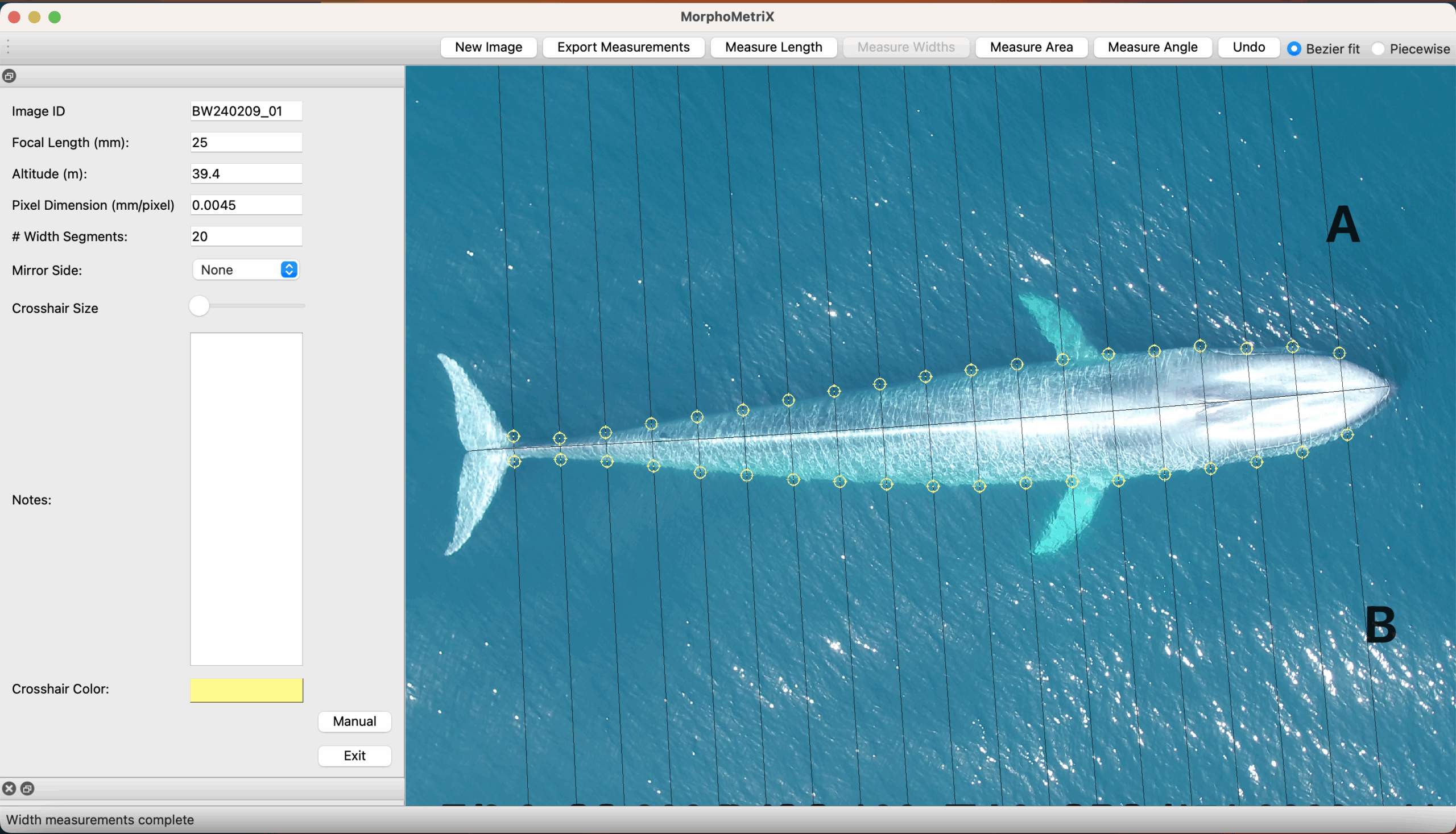
Future steps for DeteX and XtraX are to adapt the models so that measurements can be extracted from multiple whales in a single frame, which could be particularly useful for analyzing images containing mothers with their calf. We also look forward to adapting DeteX and XtraX to accommodate more species. While DeteX and XtraX was trained using only gray whale imagery, we were pleased to see that these models performed well when trialing on imagery of a blue whale (Figure 2). These results are encouraging because it shows that the models can be adapted to accommodate other species with different body shapes, such as belugas or beaked whales, with the inclusion of more training data.
We are excited to share these methods with the drone community and the rest of this blog walks through the features and steps for running DeteX and XtraX to make them even easier to use.


DeteX and XtraX walkthrough
Both DeteX and XtraX are web-based applications designed to be intuitive and user-friendly. Instructions to install and run DeteX and XtraX are available on the CODEX website. Once DeteX is launched, the default web-browser automatically opens the application where the user is asked to select 1) the folder containing the drone-based videos to analyze and 2) the folder to save output frames (Figure 3). Then, the user can select ‘start’ to begin. The default for DeteX is set to analyze the entire video from start to finish at one frame per second; if recording a video at 30 frames per second, the last (or 30th) frame is processed for each second in the video. There is also a “finetune” version of DeteX that offers users much more control, where they can change these default settings (Figure 4). For example, users can change the defaults to increase the number of frames processed per second (i.e., 10 instead of 1), to target a specific region in the video rather than the entire video, and adjust the “detection model threshold” to change the threshold of confidence the model has for detecting a whale. These specific features for enhanced control may be particularly helpful when there is a specific surfacing sequence that a user wants to have more flexibility in selecting specific frames for measuring.


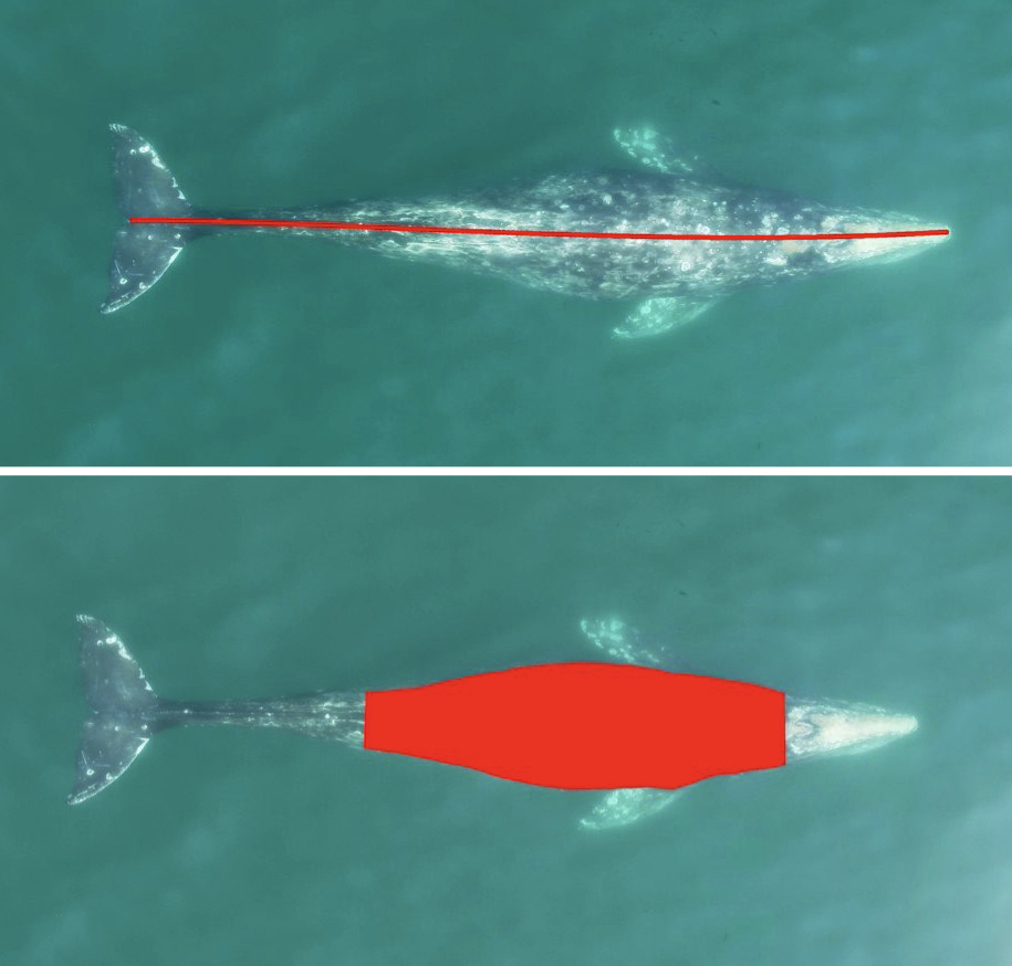
Once output frames are generated by DeteX, the user can select which frames to input into XtraX to measure. Once XtraX is launched, the default web-browser automatically opens the application where the user is asked to select 1) the folder containing the frames to measure and 2) the folder to save the output measurements. If the input frames were generated using DeteX, the barometric altitude is automatically extracted from the file name (note, that altitudes collected from a LiDAR altimeter can be joined in the XtraX output .csv file to then calculate measurements using this altitude). The image width (pixels) is automatically extracted from the input frame metadata. Users can then input specific camera parameters, such as sensor width (mm) and the focal length of the camera (mm), the launch height of the drone (i.e., if launching from hand when on a boat), and the region along the body to measure body condition (Figure 5). This region along the body is called the Head-Tail range and is identified as the area where most lipid storage takes place to estimate body condition. To run, the user selects “start”. XtraX then will output a .png file of each frame showing the keypoints (used for the body length measurement) and the shaded region (used for the body condition estimate) along the body to help visual results so users can filter for quality (Figure 6). XtraX also outputs a single .csv containing all the measurements (in meters and pixels) with their associated metadata.


We hope this walkthrough is helpful for researchers interested in using and adapting these tools for their projects. There is also a video tutorial available online. Happy (faster) measuring!
References
Bierlich, K. C., Karki, S., Bird, C. N., Fern, A., & Torres, L. G. (2024). Automated body length and body condition measurements of whales from drone videos for rapid assessment of population health. Marine Mammal Science, e13137. https://doi.org/10.1111/mms.13137
Cerini, F., Childs, D. Z., & Clements, C. F. (2023). A predictive timeline of wildlife population collapse. Nature Ecology & Evolution, 7(3), 320–331. https://doi.org/10.1038/s41559-023-01985-2