Clara Bird, PhD Student, OSU Department of Fisheries, Wildlife, and Conservation Sciences, Geospatial Ecology of Marine Megafauna Lab
When I wrote my first blog on individual specialization well over a year ago, I just skimmed the surface of the literature on this topic and only started to recognize the importance of studying individual specialization. The question, “is there individual specialization in the PCFG of gray whales?” is the focus of my first thesis chapter and the results will affect all my subsequent work. Therefore, the literature and concepts of individual specialization are a focus of my literature review and studies.
In my previous blog I focused on common characteristics of individuals that are similarly specialized as an underlying driver of individual specialization. While these characteristics (often attributable to age, sex, or physical traits) are important to consider, I’ve learned that the list of drivers of individual specialization is long and that many variables are dynamic. Of all the drivers I’ve learned about, competition is among the most common.
Competition is a major driver of individual specialization, and a common driver of competition is resource availability. When resource availability decreases, whether caused by increasing population density or changing environmental conditions, competition for that resource increases. As competition increases, individuals have a choice. They can choose to engage in competition, either by racing, fighting, or sharing [1], which can be costly, or they can diffuse the competition by focusing on a different resource. This second approach would be considered niche partitioning in the prey dimension. Niche partitioning is a way for individuals to share ecological space by using different resources. Essentially, individuals can share habitat without having to engage in direct competition by pursuing different prey types [2].
This switch to different prey types can change the degree of individual specialization present in the population (Figure 1). But the direction of the change is not constant. If all individuals were pursuing the same prey type under low competition conditions but then switched to different alternate prey types under high competition, then individual specialization would increase (Figure 1a). This direction has been observed across a range of species including sharks [3], otters [4]–[7], dolphins [8], [9], stickleback fish [10], [11], largemouth bass [12], banded mongoose [13], fur seals [14], and baleen whales [15].
However, if individuals were pursuing different prey types under low competition conditions (maybe because of underlying differences such as age or sex) but then switched to the same alternate prey types under high competition, diet overlap would increase, and individual specialization would decrease (Figure 1b). Furthermore, an individual might not switch to an entirely new prey type but instead add prey items to its diet [16]. This diet expansion under competition would also decrease individual specialization. Fewer studies have reported this direction but it’s been found in the common bumblebee [17] and in several neotropical vertebrate species [18], [19].
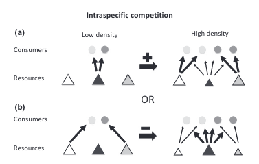
Horizontal arrows indicate the sign (positive or negative) of the effect on the degree of individual specialization. (a) Consumers share the same preferred resource (dark gray tangle) but have different alternative resources (white and light gray triangles). As the preferred resource becomes scarce, consumers switch to different alternatives, increasing the degree of individual specialization. (b) Alternatively, consumers have distinct preferred resources, so that as resources become scarce, individuals converge to the alternative resource (dark gray triangle), reducing diet variation.
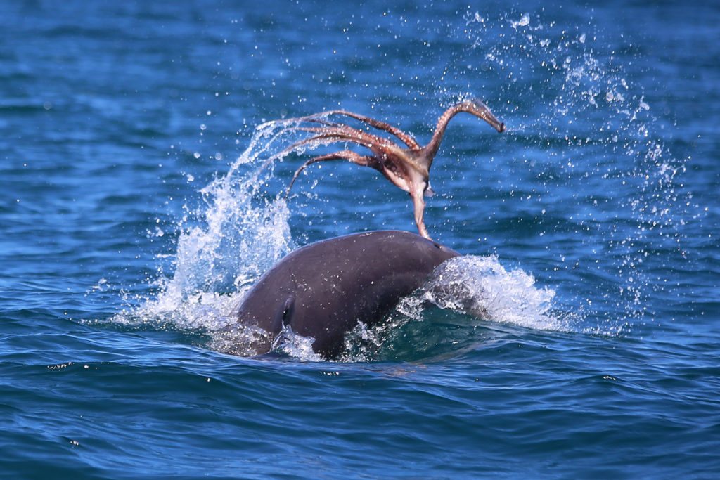
Interestingly, its hypothesized that individual specialization driven by competition is one of the factors that facilitates the formation and existence of stable groups [21]. For example, a study on resident female dolphins in Sarasota Bay, FL, USA found that females with high spatial overlap used distinct foraging specializations [8](Figure 2). This study illustrates how partitioning prey enabled spatial and social coexistence. A study on banded mongooses reached a similar conclusion [13]. They found that specialization was highest in the biggest groups (with the most competition) and not explained by sex, age, or other inherent differences. They hypothesized that specialization increasing with competition reduced conflict and allowed the groups to remain stable. This study also highlighted the role of learning to determine an individual’s specialization.

Source: https://sarasotadolphin.org
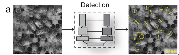
Learning drives the distribution of knowledge throughout a population, which can lead to either specialization or generalization. ‘One-to-one’ learning, where one individual learns from one demonstrator, tends to promote individual specialization [21]. This form of transmission drives specialization because the individuals who learn the specialization tend to then carry on using, and eventually teaching, that specialization [6]. A common example of ‘one-to-one’ learning is vertical transmission from parent to offspring. It has been shown to transmit specializations in dolphins [22] and otters [6]. ‘One-to-one’ learning can occur outside of parent-offspring pairs; non-parent-offspring ‘one-to-one’ learning has been shown to drive specialization in banded mongooses [13](Figure 3).
However, other forms of social learning can promote more generalized foraging strategies. ‘Many-to-one’ or ‘one-to-many’ learning can reduce the presence of specialization in species [13], [21] as can the presence of conformity in a group [23], [24].
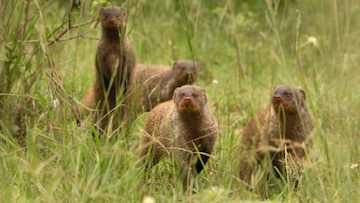
Source: http://socialisresearch.org/about-the-banded-mongoose-project/
The multiple drivers of specialization and their dynamic quality means that it is important to contextualize specialization. For example, a study on four species of neotropical frogs found varying degrees of specialization across multiple populations of each species [18]. The degree of specialization was dependent on a variety of drivers including predation and both intra- and inter-specific competition. Notably, the direction of the relationship between degree of specialization and each driver was species specific. This study highlights that one species may not always be more specialized than another, but that a populations’ specialization is context dependent.
Therefore, it is important to not only be aware of the degree of specialization present in a population, but to also understand its dynamics and drivers. These relationships can then be used to understand how, and why, a population may react to competition from other species, predators, and changes in resource availability [20]. A population’s specialization can also affect the specialization of other populations and community dynamics [25], therefore, it’s important to consider and study individual specialization on both the population and community level. I am excited to start using our incredible six-year dataset to start investigating these questions for PCFG gray whales, so stay tuned for results!
Did you enjoy this blog? Want to learn more about marine life, research, and conservation? Subscribe to our blog and get a weekly alert when we make a new post! Just add your name into the subscribe box on the left panel.
References
[1] M. Taborsky, M. A. Cant, and J. Komdeur, The Evolution of Social Behaviour. Cambridge: Cambridge University Press, 2021. doi: 10.1017/9780511894794.
[2] E. R. Pianka, “Niche Overlap and Diffuse Competition,” vol. 71, no. 5, pp. 2141–2145, 1974.
[3] P. Matich et al., “Ecological niche partitioning within a large predator guild in a nutrient-limited estuary,” Limnol. Oceanogr., vol. 62, no. 3, pp. 934–953, 2017, doi: https://doi.org/10.1002/lno.10477.
[4] S. D. Newsome et al., “The interaction of intraspecific competition and habitat on individual diet specialization: a near range-wide examination of sea otters,” Oecologia, vol. 178, no. 1, pp. 45–59, May 2015, doi: 10.1007/s00442-015-3223-8.
[5] M. T. Tinker, G. Bentall, and J. A. Estes, “Food limitation leads to behavioral diversification and dietary specialization in sea otters,” Proc. Natl. Acad. Sci., vol. 105, no. 2, pp. 560–565, Jan. 2008, doi: 10.1073/pnas.0709263105.
[6] M. T. Tinker, M. Mangel, and J. A. Estes, “Learning to be different: acquired skills, social learning, frequency dependence, and environmental variation can cause behaviourally mediated foraging specializations,” Evol. Ecol. Res., vol. 11, pp. 841–869, 2009.
[7] M. T. Tinker et al., “Structure and mechanism of diet specialisation: testing models of individual variation in resource use with sea otters,” Ecol. Lett., vol. 15, no. 5, pp. 475–483, 2012, doi: 10.1111/j.1461-0248.2012.01760.x.
[8] S. Rossman et al., “Foraging habits in a generalist predator: Sex and age influence habitat selection and resource use among bottlenose dolphins (Tursiops truncatus),” Mar. Mammal Sci., vol. 31, no. 1, pp. 155–168, 2015, doi: https://doi.org/10.1111/mms.12143.
[9] L. G. Torres, “A kaleidoscope of mammal , bird and fish : habitat use patterns of top predators and their prey in Florida Bay,” vol. 375, pp. 289–304, 2009, doi: 10.3354/meps07743.
[10] M. S. Araújo et al., “Network Analysis Reveals Contrasting Effects of Intraspecific Competition on Individual Vs. Population Diets,” Ecology, vol. 89, no. 7, pp. 1981–1993, 2008, doi: 10.1890/07-0630.1.
[11] R. Svanbäck and D. I. Bolnick, “Intraspecific competition drives increased resource use diversity within a natural population,” Proc. R. Soc. B Biol. Sci., vol. 274, no. 1611, pp. 839–844, Mar. 2007, doi: 10.1098/rspb.2006.0198.
[12] D. E. Schindler, J. R. Hodgson, and J. F. Kitchell, “Density-dependent changes in individual foraging specialization of largemouth bass,” Oecologia, vol. 110, no. 4, pp. 592–600, May 1997, doi: 10.1007/s004420050200.
[13] C. E. Sheppard et al., “Intragroup competition predicts individual foraging specialisation in a group-living mammal,” Ecol. Lett., vol. 21, no. 5, pp. 665–673, 2018, doi: 10.1111/ele.12933.
[14] L. Kernaléguen, J. P. Y. Arnould, C. Guinet, and Y. Cherel, “Determinants of individual foraging specialization in large marine vertebrates, the Antarctic and subantarctic fur seals,” J. Anim. Ecol., vol. 84, no. 4, pp. 1081–1091, 2015, doi: 10.1111/1365-2656.12347.
[15] E. M. Keen and K. M. Qualls, “Respiratory behaviors in sympatric rorqual whales: the influence of prey depth and implications for temporal access to prey,” J. Mammal., vol. 99, no. 1, pp. 27–40, Feb. 2018, doi: 10.1093/jmammal/gyx170.
[16] R. H. MacArthur and E. R. Pianka, “On Optimal Use of a Patchy Environment,” Am. Nat., vol. 100, no. 916, pp. 603–609, 1966, doi: 10.1086/282454.
[17] C. Fontaine, C. L. Collin, and I. Dajoz, “Generalist foraging of pollinators: diet expansion at high density,” J. Ecol., vol. 96, no. 5, pp. 1002–1010, 2008, doi: 10.1111/j.1365-2745.2008.01405.x.
[18] R. Costa-Pereira, V. H. W. Rudolf, F. L. Souza, and M. S. Araújo, “Drivers of individual niche variation in coexisting species,” J. Anim. Ecol., vol. 87, no. 5, pp. 1452–1464, 2018, doi: 10.1111/1365-2656.12879.
[19] M. M. Pires, P. R. Guimarães Jr, M. S. Araújo, A. A. Giaretta, J. C. L. Costa, and S. F. dos Reis, “The nested assembly of individual-resource networks,” J. Anim. Ecol., vol. 80, no. 4, pp. 896–903, 2011, doi: 10.1111/j.1365-2656.2011.01818.x.
[20] M. S. Araújo, D. I. Bolnick, and C. A. Layman, “The ecological causes of individual specialisation,”Ecol. Lett., vol. 14, no. 9, pp. 948–958, 2011, doi: https://doi.org/10.1111/j.1461-0248.2011.01662.x.
[21] C. E. Sheppard, R. Heaphy, M. A. Cant, and H. H. Marshall, “Individual foraging specialization in group-living species,” Anim. Behav., vol. 182, pp. 285–294, Dec. 2021, doi: 10.1016/j.anbehav.2021.10.011.
[22] S. Wild, S. J. Allen, M. Krützen, S. L. King, L. Gerber, and W. J. E. Hoppitt, “Multi-network-based diffusion analysis reveals vertical cultural transmission of sponge tool use within dolphin matrilines,” Biol. Lett., vol. 15, no. 7, p. 20190227, Jul. 2019, doi: 10.1098/rsbl.2019.0227.
[23] L. M. Aplin, D. R. Farine, J. Morand-Ferron, A. Cockburn, A. Thornton, and B. C. Sheldon, “Experimentally induced innovations lead to persistent culture via conformity in wild birds,” Nature, vol. 518, no. 7540, pp. 538–541, Feb. 2015, doi: 10.1038/nature13998.
[24] E. Van de Waal, C. Borgeaud, and A. Whiten, “Potent Social Learning and Conformity Shape a Wild Primate’s Foraging Decisions,” Science, Apr. 2013, doi: 10.1126/science.1232769.
[25] D. I. Bolnick et al., “Why intraspecific trait variation matters in community ecology,” Trends Ecol. Evol., vol. 26, no. 4, pp. 183–192, Apr. 2011, doi: 10.1016/j.tree.2011.01.009.