By Lisa Hildebrand, PhD student, OSU Department of Fisheries, Wildlife, & Conservation Sciences, Geospatial Ecology of Marine Megafauna Lab
Obtaining enough food is crucial for predators to ensure adequate energy gain for maintenance of vital functions and support for energetically costly life history events (e.g., reproduction). Foraging involves decisions at every step of the process, including prey selection, capture, and consumption, all of which should be as efficient as possible. Making poor foraging decisions can have long-term repercussions on reproductive success and population dynamics (Harris et al. 2007, 2008, Grémillet et al. 2008), and for marine predators that rely on prey that is spatially and temporally dynamic and notoriously patchy (Hyrenbach et al. 2000), these decisions can be especially challenging. Prey abundance and density are frequently used as predictors of marine predator distribution, movement, and foraging effort, with predators often selecting highly abundant or dense prey patches (e.g., Goldbogen et al. 2011, Torres et al. 2020). However, there is increased recognition that prey quality is also an important factor to consider when assessing a predator’s ecology and habitat use (Spitz et al. 2012), and marine predators do show a preference for higher quality prey items (e.g., Haug et al. 2002, Cade et al. 2022). Moreover, negative impacts of low-quality prey on the health and breeding success of some marine mammals (Rosen & Trites 2000, Trites & Donnelly 2003) have been documented. Therefore, examining multiple prey metrics, such as prey quantity and quality, in predator ecology studies is critical.
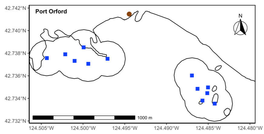
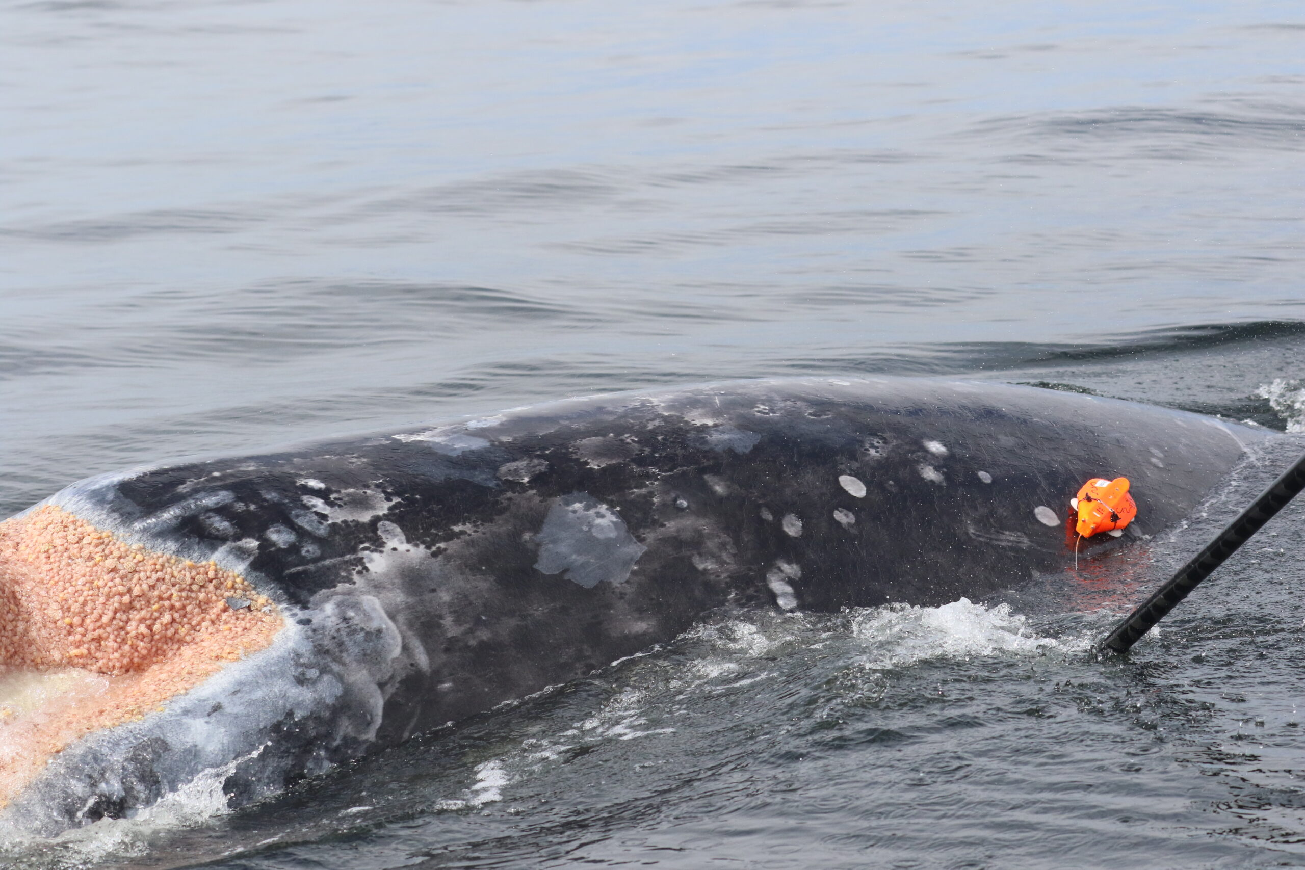
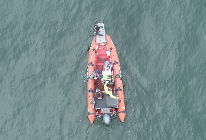
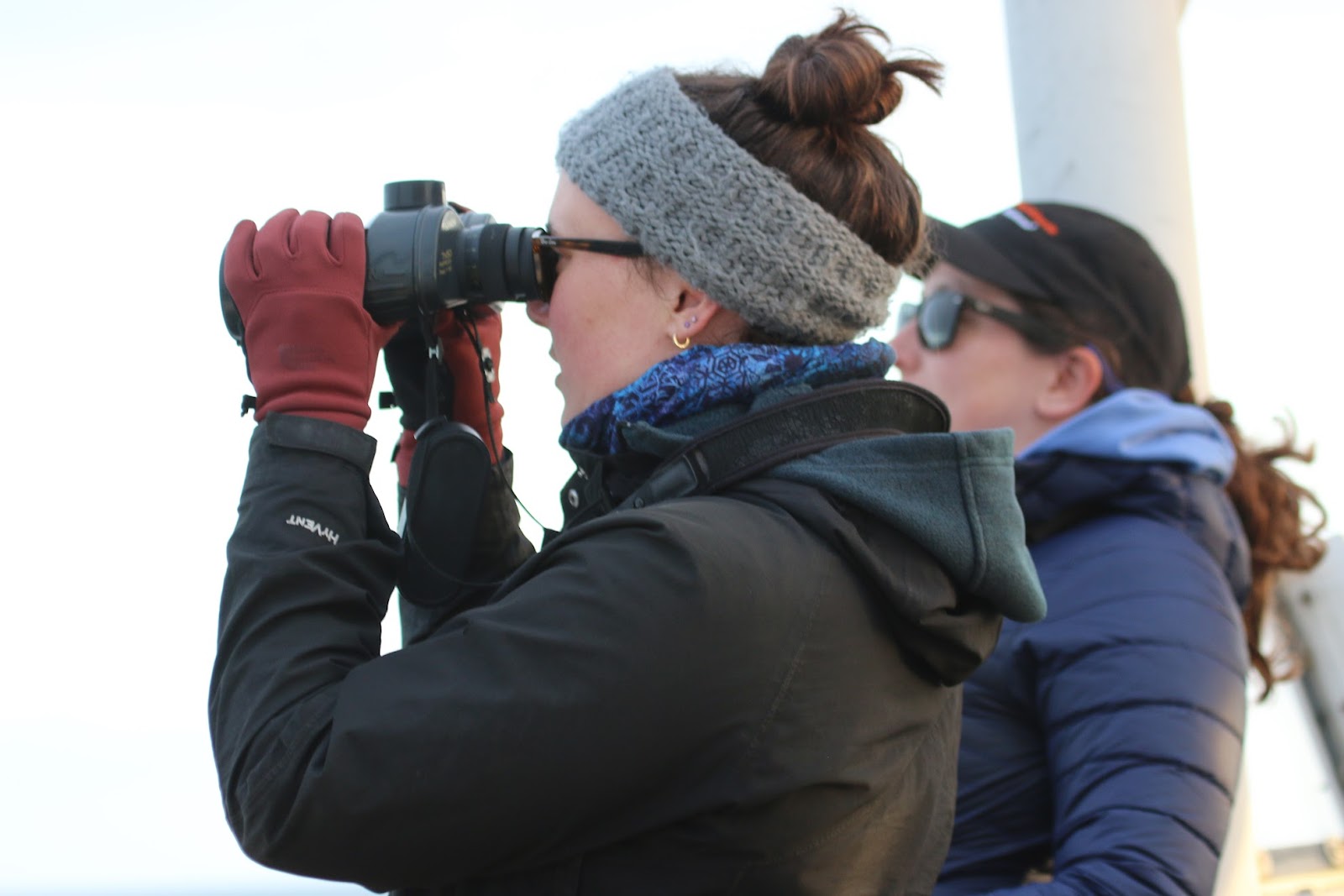
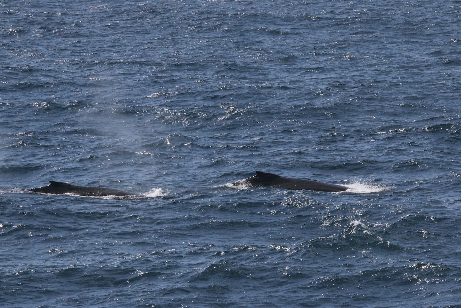
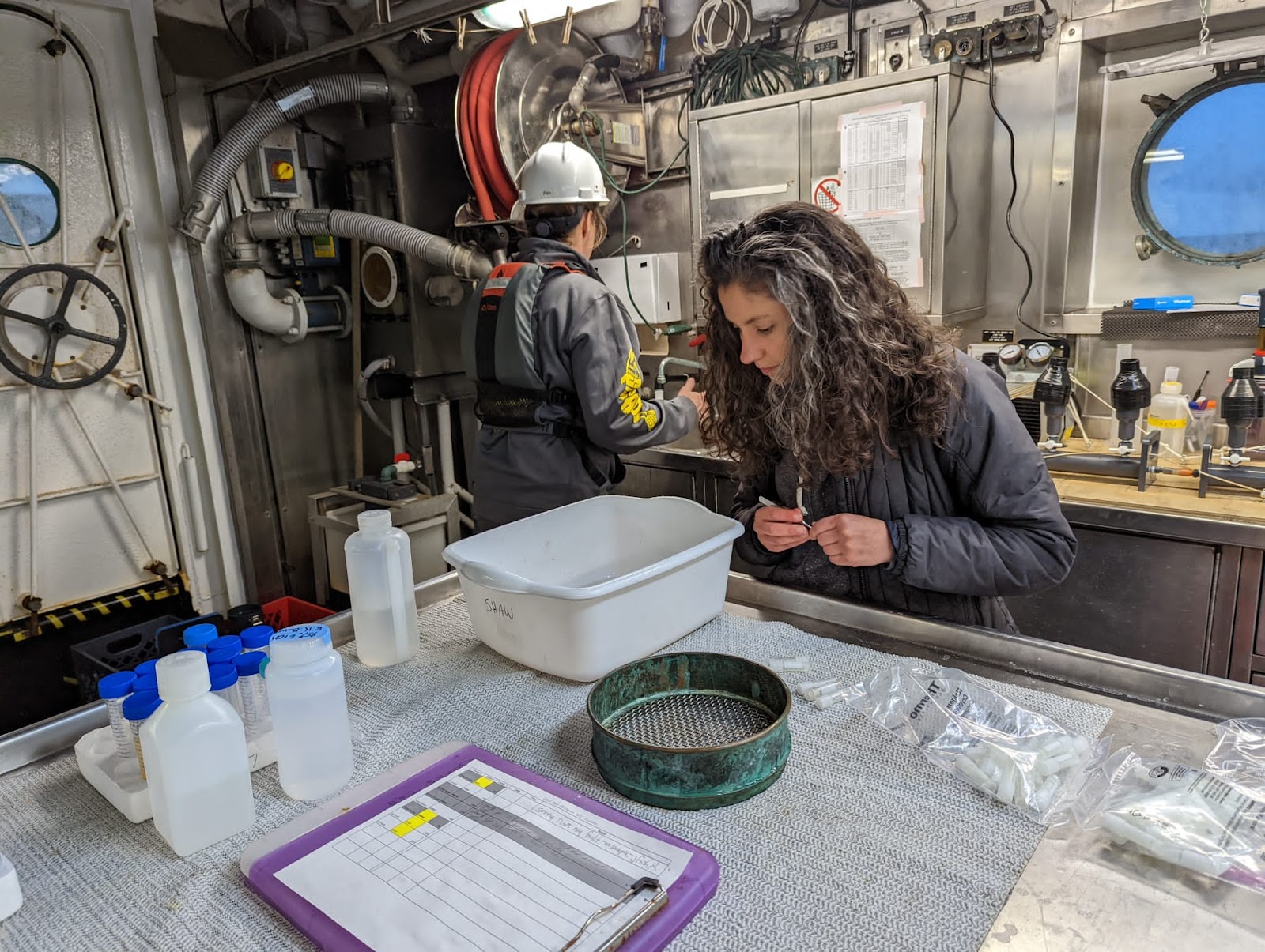
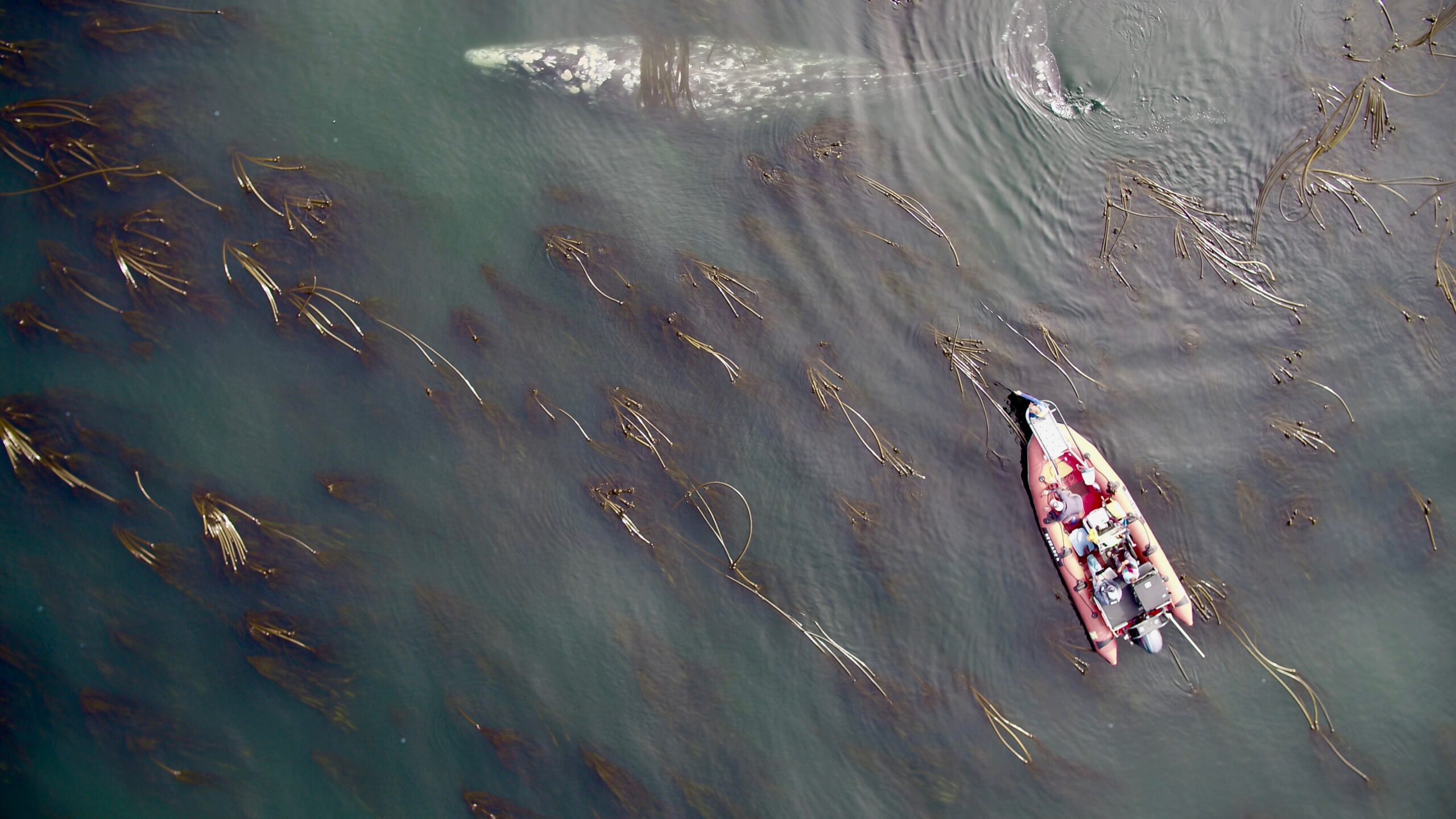
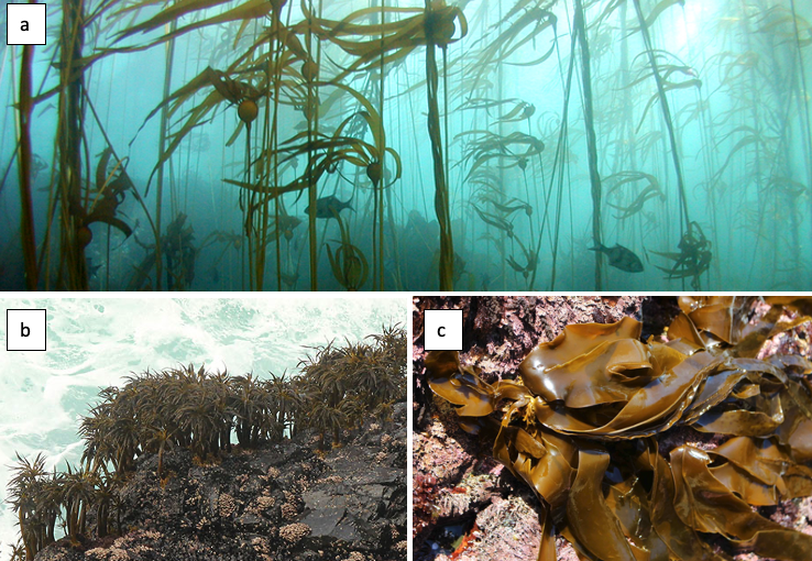
Our integrated TOPAZ/JASPER projects in Port Orford do just this! We collect both prey quantity and quality data from a tandem research kayak, while we track Pacific Coast Feeding Group (PCFG) gray whales from shore. The prey and whale sampling overlap spatially (and often temporally within the same day). This kind of concurrent predator-prey sampling at similar scales is often logistically challenging to achieve, yet because PCFG gray whales have an affinity for nearshore, coastal habitats, it is something we have been able to achieve in Port Orford. Since 2016, a field team comprised of graduate, undergraduate, and high school students has collected data during the month of August to investigate gray whale foraging decisions relative to prey. Every day, a kayak team collects GoPro videos (to assess relative prey abundance; AKA: quantity) and zooplankton samples using a tow net (to assess prey community composition; AKA: quality through caloric content of different species) (Figure 1). At the same time, a cliff team surveys for gray whales from shore and tracks them using a theodolite, which provides us with tracklines of individual whales; We categorize each location of a whale into three broad behavior states (feeding, searching, transiting) based on movement patterns. Over the years, the various students who have participated in the TOPAZ/JASPER projects have written many blog posts, which I encourage you to read here (particularly to get more detailed information about the field methods).
Several years of data are needed to conduct a robust analysis for our ecological questions about prey choice, but after seven years, we finally had the data and I am excited to share the results, which are due to the many years of hard work from many students! Our recent paper in Marine Ecology Progress Series aimed to determine whether PCFG gray whale foraging decisions are driven by prey quantity (abundance) or quality (caloric content of species) at a scale of 20 m (which is slightly less than 2 adult gray whale body lengths). In this study, we built upon results from my previous Master’s publication, which revealed that there are significant differences in the caloric content between the six common nearshore zooplankton prey species that PCFG gray whales feed on (Hildebrand et al. 2021). Therefore, in this study we addressed the hypothesis that individual whales will select areas where the prey community is dominated by the mysid shrimp Neomysis rayii, since it is significantly higher in caloric content than the other two prey species we identified, Holmesimysis sculpta (a medium quality mysid shrimp species) and Atylus tridens (a low quality amphipod species) (Hildebrand et al. 2021). We used spatial statistics and model to make daily maps of prey abundance and quality that we compared to our whale tracks and behavior from the same day. Please read our paper for the details on our novel methods that produced a dizzying amount of prey layers, which allowed us to tease apart whether gray whales target prey quantity, quality, or a mixture of both when they forage.
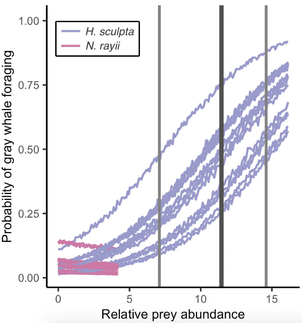
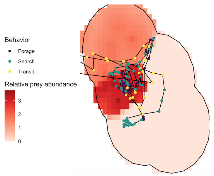
So, what did we find? The models proved our hypothesis wrong: foraging probability was significantly correlated with the quantity and quality of the mysid H. sculpta, which has significantly lower calories than N. rayii. This result puzzled us, until we started looking at the overall quantity of these two prey types in the study area and realized that the amount of calorically-rich N. rayii never reached a threshold where it was beneficial for gray whales to forage. But, there was a lot of H. sculpta, which likely made for an energetic gain for the whales despite not being as calorically rich as N. rayii. We determined a threshold of H. sculpta relative abundance that is required to initiate the gray whale foraging behavior, and the abundance of N. rayii never came close to this level (Figure 3). Despite not having the highest quality, H. sculpta did have the highest abundance and showed a significant positive relationship with foraging behavior, unlike the other prey items. Interestingly, whales never selected areas dominated by the low-calorie species A. tridens. These results demonstrate trade-off choices by whales for this abundant, medium-quality prey.
To our knowledge, individual baleen whale foraging decisions relative to available prey quantity and quality have not been addressed previously at this very fine-scale. Interestingly, this trade-off between prey quantity and quality has also been detected in humpback whales foraging in Antarctica at depths deeper than where the densest krill patches occur; while the whales are exploiting less dense krill patches, these krill composed of larger, gravid, higher-quality krill (Cade et al. 2022). While it is unclear how baleen whales differentiate between prey species or reproductive stages, several mechanisms have been suggested, including visual and auditory identification (Torres 2017). We assume here that gray whales, and other baleen whale species, can differentiate between prey species. Thus, our results showcase the importance of knowing the quality (such as caloric content) of prey items available to predators to understand their foraging ecology (Spitz et al. 2012).
References
Cade DE, Kahane-Rapport SR, Wallis B, Goldbogen JA, Friedlaender AS (2022) Evidence for size-selective pre- dation by Antarctic humpback whales. Front Mar Sci 9:747788
Goldbogen JA, Calambokidis J, Oleson E, Potvin J, Pyenson ND, Schorr G, Shadwick RE (2011) Mechanics, hydrody- namics and energetics of blue whale lunge feeding: effi- ciency dependence on krill density. J Exp Biol 214:131−146
Grémillet D, Pichegru L, Kuntz G, Woakes AG, Wilkinson S, Crawford RJM, Ryan PG (2008) A junk-food hypothesis for gannets feeding on fishery waste. Proc R Soc B 275: 1149−1156
Harris MP, Beare D, Toresen R, Nøttestad L, and others (2007) A major increase in snake pipefish (Entelurus aequoreus) in northern European seas since 2003: poten- tial implications for seabird breeding success. Mar Biol 151:973−983
Harris MP, Newell M, Daunt F, Speakman JR, Wanless S (2008) Snake pipefish Entelurus aequoreus are poor food for seabirds. Ibis 150:413−415
Haug T, Lindstrøm U, Nilssen KT (2002) Variations in minke whale (Balaenoptera acutorostrata) diet and body condi- tion in response to ecosystem changes in the Barents Sea. Sarsia 87:409−422
Hildebrand L, Bernard KS, Torres LG (2021) Do gray whales count calories? Comparing energetic values of gray whale prey across two different feeding grounds in the eastern North Pacific. Front Mar Sci 8:1008
Hyrenbach KD, Forney KA, Dayton PK (2000) Marine pro- tected areas and ocean basin management. Aquat Con- serv 10:437−458
Rosen DAS, Trites AW (2000) Pollock and the decline of Steller sea lions: testing the junk-food hypothesis. Can J Zool 78:1243−1250
Spitz J, Trites AW, Becquet V, Brind’Amour A, Cherel Y, Galois R, Ridoux V (2012) Cost of living dictates what whales, dolphins and porpoises eat: the importance of prey quality on predator foraging strategies. PLOS ONE 7:e50096
Torres LG, Barlow DR, Chandler TE, Burnett JD (2020) Insight into the kinematics of blue whale surface forag- ing through drone observations and prey data. PeerJ 8: e8906
Torres LG (2017) A sense of scale: foraging cetaceans’ use of scale-dependent multimodal sensory systems. Mar Mamm Sci 33:1170−1193
Trites AW, Donnelly CP (2003) The decline of Steller sea lions Eumetopias jubatus in Alaska: a review of the nutri- tional stress hypothesis. Mammal Rev 33:3−28