By Dr. Dawn Barlow, Postdoctoral Scholar, OSU Department of Fisheries, Wildlife, and Conservation Sciences, Geospatial Ecology of Marine Megafauna Lab
Learning by listening
Studying mobile marine animals that are only fleetingly visible from the water’s surface is challenging. However, many species including baleen whales rely on sound as a primary form of communication, producing different vocalizations related to their fundamental needs to feed and reproduce. Therefore, we can learn a lot about these elusive animals by monitoring the patterns of their calls. In the final chapter of my PhD, we set out to study blue whale ecology and life history by listening. I am excited to share our findings, recently published in Ecology and Evolution.
Blue whales produce two distinct types of vocalizations: song is produced by males and is hypothesized to play a role in breeding behavior, and D calls are a hypothesized social call produced by both sexes in association with feeding behavior. We analyzed how these different calls varied seasonally, and how they related to environmental conditions.
This paper is a collaborative study co-authored by Dr. Holger Klinck and Dimitri Ponirakis of the K. Lisa Yang Center for Conservation Bioacoustics, Dr. Trevor Branch of the University of Washington, and GEMM Lab PI Dr. Leigh Torres, and brings together multiple methods and data sources. Our findings shed light on blue whale habitat use patterns, and how climate change may impact both feeding and reproduction for this species of conservation concern.
The South Taranaki Bight: an ideal study system
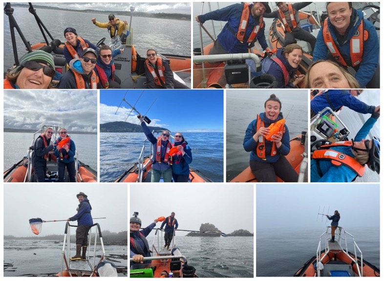
Baleen whales typically migrate between high-latitude, productive feeding grounds and low-latitude breeding grounds. However, the New Zealand blue whale population is present in the South Taranaki Bight (STB) region year-round, which uniquely enabled us to monitor their behavior, ecology, and life history across seasons and years from a single location. We recorded blue whale vocalizations from Marine Autonomous Recording Units (MARUs) deployed at five locations in the STB for two full years (Fig. 1).

We found that the two vocalization types had different seasonal occurrence patterns (Fig. 2). D calls were associated with upwelling conditions that indicate feeding opportunities, lending evidence for their function as a foraging-related call.
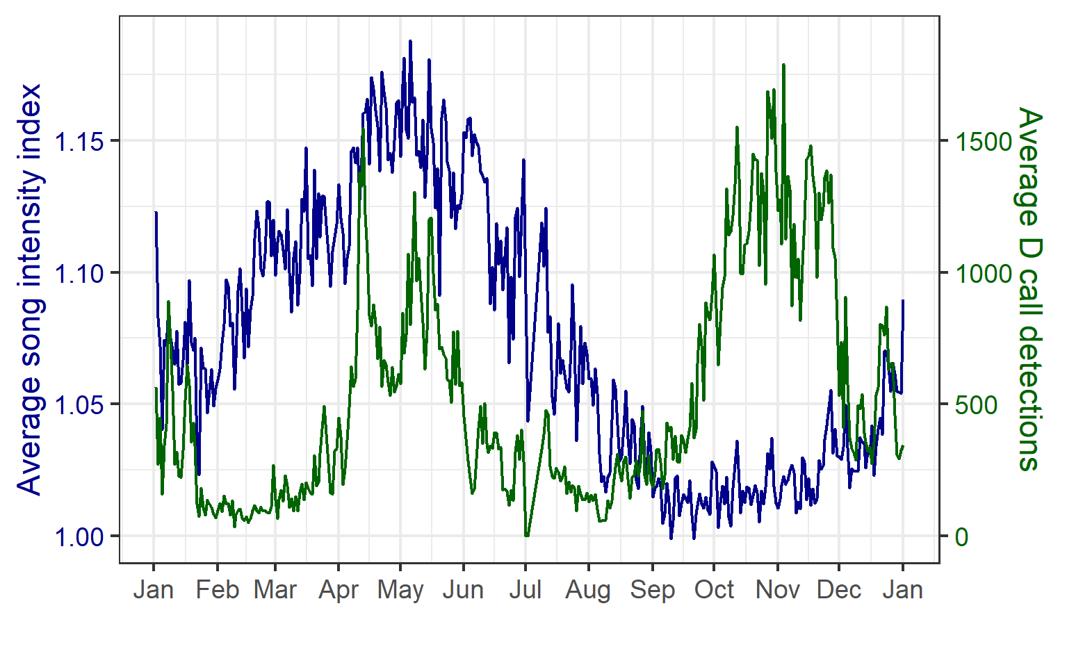
In contrast, blue whale song showed a very clear seasonal peak in the fall and was less obviously correlated with environmental conditions. To investigate the hypothesized function of song as a breeding call, we turned to a perhaps unintuitive source of information: historical whaling records. Whenever a pregnant whale was killed during commercial whaling operations, the length of the fetus was measured. By looking at the seasonal pattern in these fetal lengths, we can presume that births occur around the time of year when fetal lengths are at their longest. The records indicated April-May. By back-calculating the 11-month gestation time for a blue whale, we can presume that mating occurs generally in May-June, which is the exact time of the peak in song intensity from our recordings (Fig. 3).

With this evidence for D calls as feeding-related calls and song as breeding-related calls, we had a host of new questions, we used this gained knowledge to explore how changing environmental conditions might impact multiple life history processes for New Zealand blue whales
Marine heatwaves impact multiple life history processes
Our study period between January 2016 and February 2018 spanned both typical upwelling conditions and dramatic marine heatwaves in the STB region. While we previously documented that the marine heatwave of 2016 affected blue whale distribution, the population-level impacts on feeding and reproductive effort remained unknown. In our recent study, we found that during marine heatwaves, D calls were dramatically reduced compared to during productive upwelling conditions. During the fall breeding peak, song intensity was likewise dramatically reduced following the marine heatwave. This relationship indicates that following poor feeding conditions, blue whales may invest less effort in reproduction. As marine heatwaves are projected to become more frequent and more intense under global climate change, our findings are perhaps a warning for what is to come as animal populations must contend with changing ocean conditions.
More than a decade of research on New Zealand blue whales
Ten years ago, Leigh first put forward a hypothesis that the STB region was an undocumented blue whale foraging ground based on multiple lines of evidence (Torres 2013). Despite pushback and numerous challenges, Leigh set out to prove her hypothesis through a comprehensive, multi-year data collection effort. I was lucky enough to join the team in 2016, first as a Masters’ student, and then as a PhD student. In the time since Leigh’s hypothesis, we not only documented the New Zealand blue whale population (Barlow et al. 2018), we learned a great deal about what drives blue whale feeding behavior (Torres et al. 2020) and habitat use patterns (Barlow et al. 2020, 2021), and developed forecast models to predict blue whale distribution for dynamic management of the STB (Barlow & Torres 2021). We also documented their unique, year-round presence in the STB, distinct from the migratory or vagrant presence of other blue whale populations (Barlow et al. 2022b). We now understand how marine heatwaves impact both feeding opportunities and reproductive effort (Barlow et al. 2023). We even analyzed blue whale skin condition (Barlow et al. 2019) and acoustic response to earthquakes (Barlow et al. 2022a) along the way. A decade later, it is humbling to reflect on how much we have learned about these whales. This paper is also the final chapter of my PhD, and as I reflect on how I have grown both personally and scientifically since I interviewed with Leigh as a wide-eyed undergraduate student in fall 2015, I am filled with gratitude for the opportunities for learning and growth that Leigh, these whales, and many mentors and collaborators have offered over the years. As is often the case in science, the more questions you ask, the more questions you end up with. We are already dreaming up future studies to further understand the ecology, health, and resilience of this blue whale population. I can only imagine what we might learn in another decade.

Did you enjoy this blog? Want to learn more about marine life, research, and conservation? Subscribe to our blog and get a weekly alert when we make a new post! Just add your name into the subscribe box below!
References:
Barlow DR, Bernard KS, Escobar-Flores P, Palacios DM, Torres LG (2020) Links in the trophic chain: Modeling functional relationships between in situ oceanography, krill, and blue whale distribution under different oceanographic regimes. Mar Ecol Prog Ser 642:207–225.
Barlow DR, Estrada Jorge M, Klinck H, Torres LG (2022a) Shaken, not stirred: blue whales show no acoustic response to earthquake events. R Soc Open Sci 9:220242.
Barlow DR, Klinck H, Ponirakis D, Branch TA, Torres LG (2023) Environmental conditions and marine heatwaves influence blue whale foraging and reproductive effort. Ecol Evol 13:e9770.
Barlow DR, Klinck H, Ponirakis D, Garvey C, Torres LG (2021) Temporal and spatial lags between wind, coastal upwelling, and blue whale occurrence. Sci Rep 11:1–10.
Barlow DR, Klinck H, Ponirakis D, Holt Colberg M, Torres LG (2022b) Temporal occurrence of three blue whale populations in New Zealand waters from passive acoustic monitoring. J Mammal.
Barlow DR, Pepper AL, Torres LG (2019) Skin deep: An assessment of New Zealand blue whale skin condition. Front Mar Sci 6:757.
Barlow DR, Torres LG (2021) Planning ahead: Dynamic models forecast blue whale distribution with applications for spatial management. J Appl Ecol 58:2493–2504.
Barlow DR, Torres LG, Hodge KB, Steel D, Baker CS, Chandler TE, Bott N, Constantine R, Double MC, Gill P, Glasgow D, Hamner RM, Lilley C, Ogle M, Olson PA, Peters C, Stockin KA, Tessaglia-hymes CT, Klinck H (2018) Documentation of a New Zealand blue whale population based on multiple lines of evidence. Endanger Species Res 36:27–40.
Torres LG (2013) Evidence for an unrecognised blue whale foraging ground in New Zealand. New Zeal J Mar Freshw Res 47:235–248.
Torres LG, Barlow DR, Chandler TE, Burnett JD (2020) Insight into the kinematics of blue whale surface foraging through drone observations and prey data. PeerJ 8:e8906.