Sagar Karki, Master’s student in the Computer Science Department at Oregon State University
What beasts? Good question! We are talking about gray whales in this article but honestly we can tweak the system discussed in this blog a little and make it usable for other marine animals too.
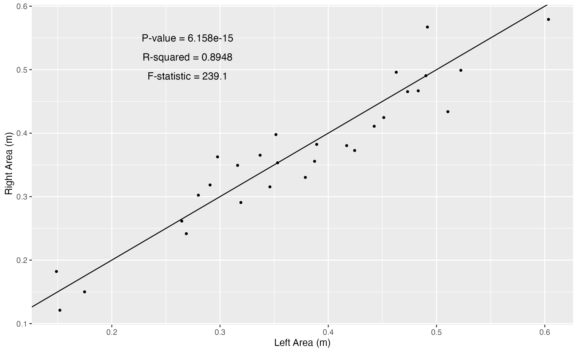
Understanding the morphology, such as body area and length, of wild animals and populations can provide important information on animal behavior and health (check out postdoc Dr. KC Bierlich’s post on this topic). Since 2015, the GEMM Lab has been flying drones over whales to collect aerial imagery to allow for photogrammetric measurements to gain this important morphological data. This photogrammetry data has shed light on multiple important aspects of gray whale morphology, including the facts that the whales feeding off Oregon are skinnier [1] and shorter [2] than the gray whales that feed in the Arctic region. But, these surprising conclusions overshadow the immense, time-consuming labor that takes place behind the scenes to move from aerial images to accurate measurements.
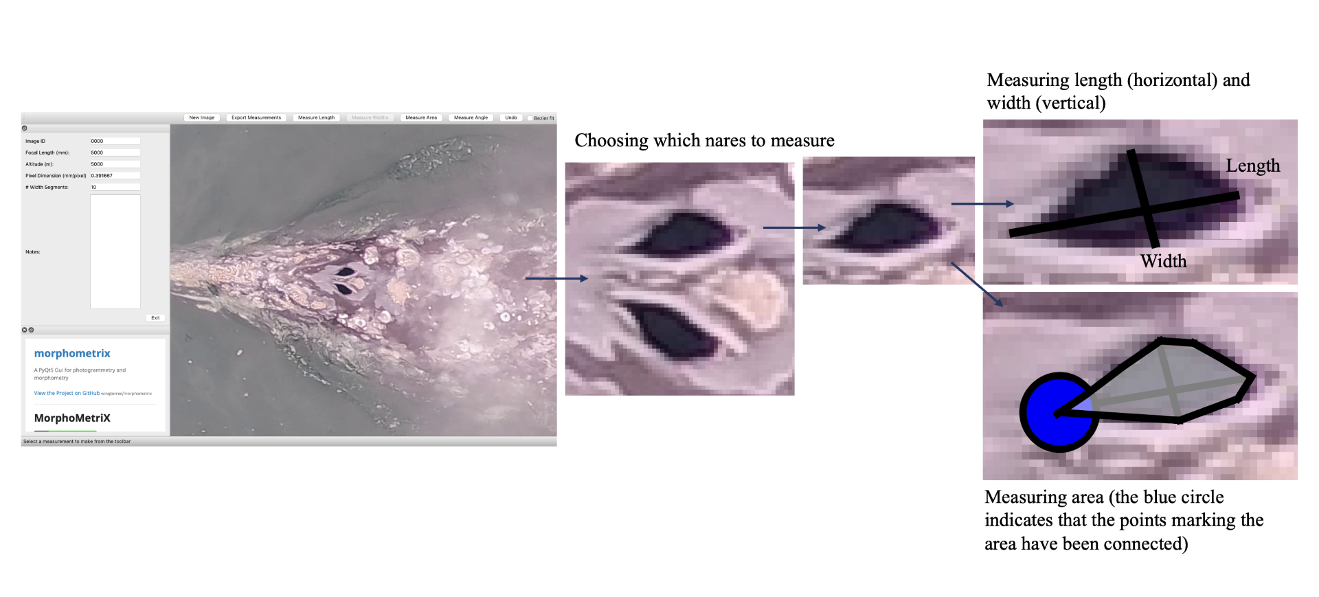
To give you a sense of this laborious process, here is a quick run through of the methods: First the 10 to 15 minute videos must be carefully watched to select the perfect frames of a whale (flat and straight at the surface) for measurement. The selected frames from the drone imagery are then imported into MorphoMetriX, which is a custom software developed for photogrammetry measurement [1]. MorphoMetriX is an interactive application that allows an analyst to manually measure the length by clicking points along the centerline of the whale’s body. Based on this line, the whale is divided into a set of sections perpendicular to the centerline, these are used to then measure widths along the body. The analyst then clicks border points at the edge of the whale’s body to delineate the widths following the whale’s body curve. MorphoMetriX then generates a file containing the lengths and widths of the whale in pixels for each measured image. The length and widths of whales are converted from pixels to metric units using a software called CollatriX [4] and this software also calculates metrics of body condition from the length and width measurements.
While MorphoMetriX [3] and CollatriX [4] are both excellent platforms to facilitate these photogrammetry measurements, each measurement takes time, a keen eye, and attention to detail. Plus, if you mess up one step, such as an incorrect length or width measurement, you have to start from the first step. This process is a bottleneck in the process of obtaining important morphology data on animals. Can we speed this process up and still obtain reliable data?
What if we can apply automation using computer vision to extract the frames we need and automatically obtain measurements that are as accurate as humans can obtain? Sounds pretty nice, huh? This is where I come into the picture. I am a Master’s student in the Computer Science Department at OSU, so I lack a solid background in marine science, but bring to the table my skills as a computer programmer. For my master’s project, I have been working in the GEMM Lab for the past year to develop automated methods to obtain accurate photogrammetry measurements of whales.
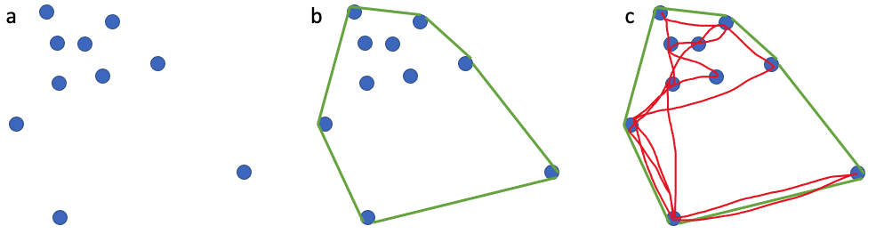
We are not the first group to attempt to use computers and AI to speed up and improve the identification and detection of whales and dolphins in imagery. Researchers have used deep learning networks to speed up the time-intensive and precise process of photo-identification of individual whales and dolphins [5], allowing us to more quickly determine animal location, movements and abundance. Millions of satellite images of the earth’s surface are collected daily and scientists are attempting to utilize these images to benefit marine life by studying patterns of species occurrence, including detection of gray whales in satellite images using deep learning [6]. There has also been success using computer vision to identify whale species and segment out the body area of the whales from drone imagery [7]. This process involves extracting segmentation masks of the whale’s body followed by length extraction from the mask. All this previous research shows promise for the application of computer vision and AI to assist with animal research and conservation. As discussed earlier, the automation of image extraction and photogrammetric measurement from drone videos will help researchers collect vital data more quickly so that decisions that impact the health of whales can be more responsive and effective.For instance, photogrammetry data extracted from drone images can diagnose pregnancy of the whales [8], thus automation of this information could speed up our ability to understand population trends.
Computer vision and natural language processing fields are growing exponentially. There are new foundation models like ChatGPT that can do most of the natural language understanding and processing tasks. Foundational models are also emerging for computer vision tasks, such as “the segment anything model” from Meta. Using these foundation models along with other existing research work in computer vision, we have developed and deployed a system that automates the manual and computational tasks of MorphoMetriX and CollatriX systems.
This system is currently in its testing and monitoring phase, but we are rapidly moving toward a publication to disseminate all the tools developed, so stay tuned for the research paper that will explain in detail the methodologies followed on data processing, model training and test results. The following images give a sneak peak of results. Each image illustrates a frame from a drone video that was identified and extracted through automation, followed by another automation process that identified important points along the whale’s body and curvature. The user interface of the system aims to make the user experience intuitive and easy to follow. The deployment is carefully designed to run on different hardwares, with easy monitoring and update options using the latest open source frameworks. The user has to do just two things. First, select the videos for analysis. The system then generates potential frames for photogrammetric analysis (you don’t need to watch 15 mins of drone footage!). Second, the user selects the frame of choice for photogrammetric analysis and waits for the system to give you measurements. Simple! Our goal is for these softwares to be a massive time-saver while still providing vital, accurate body measurements to the researchers in record time. Furthermore, an advantage of this approach is that researchers can follow the methods in our to-be-soon-published research paper to make a few adjustments enabling the software to measure other marine species, thus expanding the impact of this work to many other life forms.


Did you enjoy this blog? Want to learn more about marine life, research, and conservation? Subscribe to our blog and get a weekly message when we post a new blog. Just add your name and email into the subscribe box below.
References
- Torres LG, Bird CN, Rodríguez-González F, Christiansen F, Bejder L, Lemos L, Urban R J, Swartz S, Willoughby A, Hewitt J, Bierlich K (2022) Range-Wide Comparison of Gray Whale Body Condition Reveals Contrasting Sub-Population Health Characteristics and Vulnerability to Environmental Change. Front Mar Sci 910.3389/fmars.2022.867258
- Bierlich KC, Kane A, Hildebrand L, Bird CN, Fernandez Ajo A, Stewart JD, Hewitt J, Hildebrand I, Sumich J, Torres LG (2023) Downsized: gray whales using an alternative foraging ground have smaller morphology. Biol Letters 19:20230043 doi:10.1098/rsbl.2023.0043
- Torres et al., (2020). MorphoMetriX: a photogrammetric measurement GUI for morphometric analysis of megafauna. Journal of Open Source Software, 5(45), 1825, https://doi.org/10.21105/joss.01825
- Bird et al., (2020). CollatriX: A GUI to collate MorphoMetriX outputs. Journal of Open Source Software, 5(51), 2328, https://doi.org/10.21105/joss.02328
- Patton, P. T., Cheeseman, T., Abe, K., Yamaguchi, T., Reade, W., Southerland, K., Howard, A., Oleson, E. M., Allen, J. B., Ashe, E., Athayde, A., Baird, R. W., Basran, C., Cabrera, E., Calambokidis, J., Cardoso, J., Carroll, E. L., Cesario, A., Cheney, B. J. … Bejder, L. (2023). A deep learning approach to photo–identification demonstrates high performance on two dozen cetacean species. Methods in Ecology and Evolution, 00, 1–15. https://doi.org/10.1111/2041-210X.14167
- Green, K.M., Virdee, M.K., Cubaynes, H.C., Aviles-Rivero, A.I., Fretwell, P.T., Gray, P.C., Johnston, D.W., Schönlieb, C.-B., Torres, L.G. and Jackson, J.A. (2023), Gray whale detection in satellite imagery using deep learning. Remote Sens Ecol Conserv. https://doi.org/10.1002/rse2.352
- Gray, PC, Bierlich, KC, Mantell, SA, Friedlaender, AS, Goldbogen, JA, Johnston, DW. Drones and convolutional neural networks facilitate automated and accurate cetacean species identification and photogrammetry. Methods Ecol Evol. 2019; 10: 1490–1500. https://doi.org/10.1111/2041-210X.13246
- Fernandez Ajó A, Pirotta E, Bierlich KC, Hildebrand L, Bird CN, Hunt KE, Buck CL, New L, Dillon D, Torres LG (2023) Assessment of a non-invasive approach to pregnancy diagnosis in gray whales through drone-based photogrammetry and faecal hormone analysis. Royal Society Open Science 10:230452