Dr. KC Bierlich, Postdoctoral Scholar, OSU Department of Fisheries, Wildlife, & Conservation Sciences, Geospatial Ecology of Marine Megafauna Lab
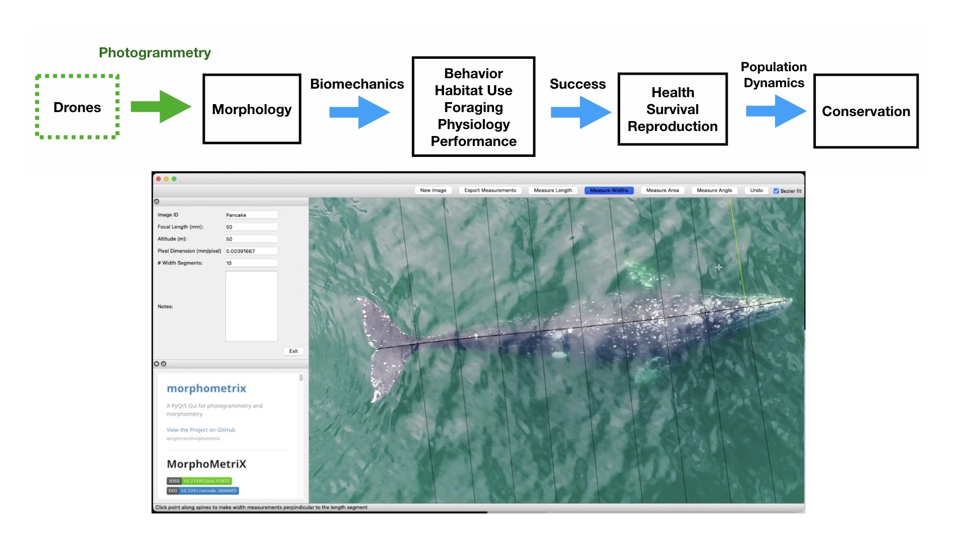
The morphology and body size of an animal is one of the most fundamental factors for understanding a species ecology. For instance, fish body size and fin shape can influence its habitat use, foraging behavior, prey type, physiological performance, and predator avoidance strategies (Fig 1). Morphology and body size can thus reflect details of an individual’s current health, likelihood of survival, and potential reproductive success, which directly influences a species life history patterns, such as reproductive status, growth rate, and energetic requirements. Collecting accurate morphological measurements of individuals is often essential for monitoring populations, and recent studies have demonstrated how animal morphology has profound implications for conservation and management decisions, especially for populations inhabiting anthropogenically-altered environments (Miles 2020) (Fig. 1). For example, in a study on the critically endangered European eel, De Meyer et al. (2020) found that different skulls sizes were associated with different ecomorphs (a local variety of a species whose appearance is determined by its ecological environment), which predicted different diet types and resulted with some ecomorphs having a greater exposure to pollutants and toxins than others. However, obtaining manual measurements of wild animal populations can be logistically challenging, limited by accessibility, cost, danger, and animal disturbance. These challenges are especially true for large elusive animals, such as whales that are often in remote locations, spend little time at the surface of the water, and their large size can preclude safe capture and live handling.

Photogrammetry is a non-invasive method for obtaining accurate morphological measurements of animals from photographs. The two main types of photogrammetry methods used in wildlife biology are 1) single camera photogrammetry, where a known scale factor is applied to a single image to measure 2D distances and angles and 2) stereo-photogrammetry, where two or more images (from a single or multiple cameras) are used to recreate 3D models. These techniques have been used on domestic animals to measure body condition and estimate weight of dairy cows and lactating Mediterranean buffaloes (Negretti et al., 2008; Gaudioso et al., 2014) and on wild animals to measure sexual dimorphism in Western gorillas (Breuer et al., 2007), shoulder heights of elephants (Schrader et al., 2006), nutritional status of Japanese macaques (Kurita et al., 2012), and the body condition of brown bears (Shirane et al., 2020). Over 70 years ago, Leedy (1948) encouraged wildlife biologists to use aerial photogrammetry from aircraft for censusing wild animal populations and their habitats, where photographs can be collected at nadir (straight down) or an oblique angle, and the scale can be calculated by dividing the focal length of the camera by the altitude or by using a ratio of selected points in an image of a known size. Indeed, aerial photogrammetry has been wildly adopted by wildlife biologists and has proven useful in obtaining measurements in large vertebrates, such as elephants and whales.
Whitehead & Payne (1978) first demonstrated the utility of using aerial photogrammetry from airplanes and helicopters as a non-invasive technique for estimating the body length of southern right whales. Prior to this technique, measurements of whales were traditionally limited to assessing carcasses collected from scientific whaling operations, or opportunistically from commercial whaling, subsistence hunting, stranding events, and bycatch. Importantly, aerial photogrammetry provides a method to collect measurements of whales without killing them. This approach has been widely adopted to obtain body length measurements on a variety of whale and dolphin species, including bowhead whales (Cubbage & Calambokidis, 1987), southern right whales (Best & Rüther, 1992), fin whales (Ratnaswamy and Wynn, 1993), common dolphins (Perryman and Lynn, 1993), spinner dolphins (Perryman & Westlake 1998), and killer whales (Fearnbach et al. 2012). Aerial photogrammetry has also been used to measure body widths to estimate nutritive condition related to reproduction in gray whales (Perryman and Lynn, 2002) and northern and southern right whales (Miller et al., 2012). However, these studies collected photographs from airplanes and helicopters, which can be costly, limited by weather and infrastructure to support aircraft research efforts and, importantly, presents a potential risk to wildlife biologists (Sasse 2003).
The recent advancement and commercialization of unoccupied aircraft systems (UAS, or drones) has revolutionized the ability to obtain morphological measurements from high resolution aerial photogrammetry across a variety of ecosystems (Fig. 2). Drones ultimately bring five transformative qualities to conservation science compared to airplanes and helicopters: affordability, immediacy, quality, efficiency, and safety of data collection. Durban et al. (2015) first demonstrated the utility of using drones for non-invasively obtaining morphological measurements of killer whales in remote environments. Since then, drone-based morphological measurements have been applied to a wide range of studies that have increased our understanding on different whale populations. For example, Leslie et al. (2020) used drone-based measurements of the skull to distinguish a unique sub-species of blue whales off the coast of Chile. Groskreutz et al. (2019) demonstrated how long-term nutritional stress has limited body growth in northern resident killer whales, while Stewart et al. (2021) found a decrease in body length of North Atlantic Right whales since 1981 that was associated with entanglements from fishing gear and may be a contributing factor to the decrease in reproductive success for this endangered population.
Drone imagery is commonly used to estimate the body condition of baleen whales by measuring the body length and width of individuals. Recently, the GEMM Lab used body length and width measurements to quantify intra- and inter-seasonal changes in body condition across individual gray whales (Lemos et al., 2020). Drones have also been used to measure body condition loss in humpback whales during the breeding season (Christiansen et al., 2016) and to compare the healthy southern right whales to the skinnier, endangered North Atlantic right whales (Christiansen et al., 2020). Drone-based assessments of body condition have even been used to measure how calf growth rate is directly related to maternal loss during suckling (Christiansen et al., 2018), and even estimate body mass (Christiansen et al., 2019).
Drone-based morphological measurements can also be combined with whale-borne inertial sensing tag data to study the functional morphology across several different baleen whale species. Kahane-Rapport et al. (2020) used drone measurements of tagged whales to analyze the biomechanics of how larger whales require longer times for filtering the water through their baleen when feeding. Gough et al. (2019) used size measurements from drones and swimming speeds from tags to determine that a whale’s “walking speed” is 2 meters per second – whether the largest of the whales, a blue whale, or the smallest of the baleen whales, an Antarctic minke whale. Size measurements and tag data were combined by Segre et al. (2019) to quantify the energetic costs of different sized whales when breaching.
Taken together, drones have revolutionized our ability to obtain morphological measurements of whales, greatly increasing our capacity to better understand how these animals function and perform in their environments. These advancements in marine science are particularly important as these methods provide greater opportunity to monitor the health of populations, especially as they face increased threats from anthropogenic stressors (such as vessel traffic, ocean noise, pollution, fishing entanglement, etc.) and climate change.
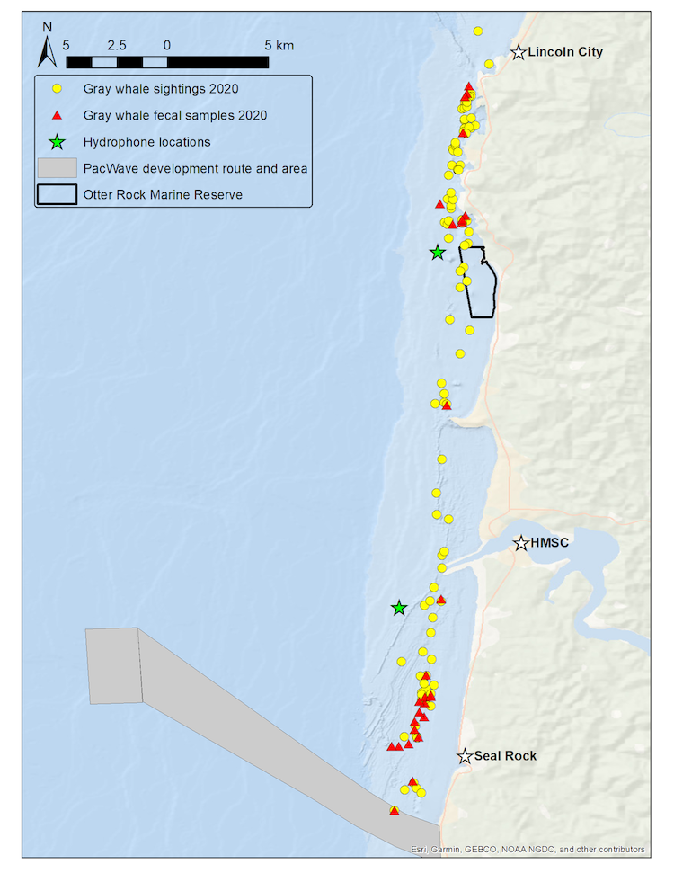
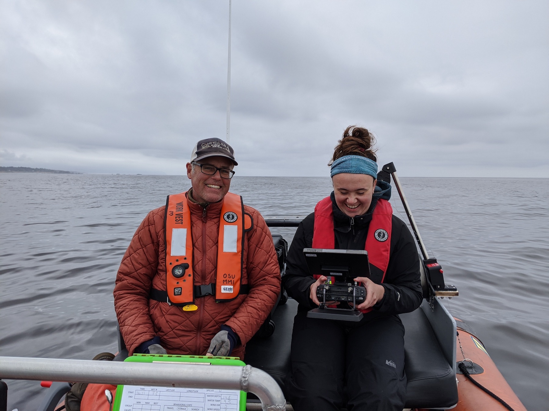
Drone-based photogrammetry is one of the main focuses of the GEMM Lab’s project on Gray whale Response to Ambient Noise Informed by Technology and Ecology (GRANITE). This summer we have been collecting drone videos to measure the body condition of gray whales feeding off the coast of Newport, Oregon (Fig. 2). As we try to understand the physiological stress response of gray whales to noise and other potential stressors, we have to account for the impacts of overall nutritional state of each individual whale’s physiology, which we infer from these body condition estimates.
References
Best, P. B., & Rüther, H. (1992). Aerial photogrammetry of southern right whales, Eubalaena australis. Journal of Zoology, 228(4), 595-614.
Breuer, T., Robbins, M. M., & Boesch, C. (2007). Using photogrammetry and color scoring to assess sexual dimorphism in wild western gorillas (Gorilla gorilla). American Journal of Physical Anthropology, 134(3), 369–382. https://doi.org/10.1002/ajpa.20678
Christiansen, F., Vivier, F., Charlton, C., Ward, R., Amerson, A., Burnell, S., & Bejder, L. (2018). Maternal body size and condition determine calf growth rates in southern right whales. Marine Ecology Progress Series, 592, 267–281.
Christiansen, F. (2020). A population comparison of right whale body condition reveals poor state of North Atlantic right whale, 1–43.
Christiansen, F., Dujon, A. M., Sprogis, K. R., Arnould, J. P. Y., & Bejder, L. (2016). Noninvasive unmanned aerial vehicle provides estimates of the energetic cost of reproduction in humpback whales. Ecosphere, 7(10), e01468–18.
Christiansen, F., Sironi, M., Moore, M. J., Di Martino, M., Ricciardi, M., Warick, H. A., … Uhart, M. M. (2019). Estimating body mass of free-living whales using aerial photogrammetry and 3D volumetrics. Methods in Ecology and Evolution, 10(12), 2034–2044.
Cubbage, J. C., & Calambokidis, J. (1987). Size-class segregation of bowhead whales discerned through aerial stereo-photogrammetry. Marine Mammal Science, 3(2), 179–185.
De Meyer, J., Verhelst, P., & Adriaens, D. (2020). Saving the European Eel: How Morphological Research Can Help in Effective Conservation Management. Integrative and Comparative Biology, 23, 347–349.
Gaudioso, V., Sanz-Ablanedo, E., Lomillos, J. M., Alonso, M. E., Javares-Morillo, L., & Rodr\’\iguez, P. (2014). “Photozoometer”: A new photogrammetric system for obtaining morphometric measurements of elusive animals, 1–10.
Gough, W. T., Segre, P. S., Bierlich, K. C., Cade, D. E., Potvin, J., Fish, F. E., … Goldbogen, J. A. (2019). Scaling of swimming performance in baleen whales. Journal of Experimental Biology, 222(20), jeb204172–11.
Groskreutz, M. J., Durban, J. W., Fearnbach, H., Barrett-Lennard, L. G., Towers, J. R., & Ford, J. K. B. (2019). Decadal changes in adult size of salmon-eating killer whales in the eastern North Pacific. Endangered Species Research, 40, 1
Kahane-Rapport, S. R., Savoca, M. S., Cade, D. E., Segre, P. S., Bierlich, K. C., Calambokidis, J., … Goldbogen, J. A. (2020). Lunge filter feeding biomechanics constrain rorqual foraging ecology across scale. Journal of Experimental Biology, 223(20), jeb224196–8.
Leedy, D. L. (1948). Aerial Photographs, Their Interpretation and Suggested Uses in Wildlife Management. The Journal of Wildlife Management, 12(2), 191.
Lemos, L. S., Burnett, J. D., Chandler, T. E., Sumich, J. L., and Torres, L. G. (2020). Intra- and inter-annual variation in gray whale body condition on a foraging ground. Ecosphere 11.
Leslie, M. S., Perkins-Taylor, C. M., Durban, J. W., Moore, M. J., Miller, C. A., Chanarat, P., … Apprill, A. (2020). Body size data collected non-invasively from drone images indicate a morphologically distinct Chilean blue whale (Balaenoptera musculus) taxon. Endangered Species Research, 43, 291–304.
Miles, D. B. (2020). Can Morphology Predict the Conservation Status of Iguanian Lizards? Integrative and Comparative Biology.
Miller, C. A., Best, P. B., Perryman, W. L., Baumgartner, M. F., & Moore, M. J. (2012). Body shape changes associated with reproductive status, nutritive condition and growth in right whales Eubalaena glacialis and E. australis. Marine Ecology Progress Series, 459, 135–156.
Negretti, P., Bianconi, G., Bartocci, S., Terramoccia, S., & Verna, M. (2008). Determination of live weight and body condition score in lactating Mediterranean buffalo by Visual Image Analysis. Livestock Science, 113(1), 1–7. https://doi.org/10.1016/j.livsci.2007.05.018
Ratnaswamy, M. J., & Winn, H. E. (1993). Photogrammetric Estimates of Allometry and Calf Production in Fin Whales, \emph{Balaenoptera physalus}. American Society of Mammalogists, 74, 323–330.
Perryman, W. L., & Lynn, M. S. (1993). Idendification of geographic forms of common dolphin(\emph{Delphinus Delphis}) from aerial photogrammetry. Marine Mammal Science, 9(2), 119–137.
Perryman, W. L., & Lynn, M. S. (2002). Evaluation of nutritive condition and reproductive status of migrating gray whales (\emph{Eschrichtius robustus}) based on analysisof photogrammetric data. Journal Cetacean Research and Management, 4(2), 155–164.
Perryman, W. L., & Westlake, R. L. (1998). A new geographic form of the spinner dolphin, stenella longirostris, detected with aerial photogrammetry. Marine Mammal Science, 14(1), 38–50.
Sasse, B. (2003). Job-Related Mortality of Wildlife Workers in the United States, 1937- 2000, 1015–1020.
Segre, P. S., Potvin, J., Cade, D. E., Calambokidis, J., Di Clemente, J., Fish, F. E., … & Goldbogen, J. A. (2020). Energetic and physical limitations on the breaching performance of large whales. Elife, 9, e51760.
Shirane, Y., Mori, F., Yamanaka, M., Nakanishi, M., Ishinazaka, T., Mano, T., … Shimozuru, M. (2020). Development of a noninvasive photograph-based method for the evaluation of body condition in free-ranging brown bears. PeerJ, 8, e9982. https://doi.org/10.7717/peerj.9982
Shrader, A. M., M, F. S., & Van Aarde, R. J. (2006). Digital photogrammetry and laser rangefinder techniques to measure African elephants, 1–7.
Stewart, J. D., Durban, J. W., Knowlton, A. R., Lynn, M. S., Fearnbach, H., Barbaro, J., … & Moore, M. J. (2021). Decreasing body lengths in North Atlantic right whales. Current Biology.
Walker, J. A., Alfaro, M. E., Noble, M. M., & Fulton, C. J. (2013). Body fineness ratio as a predictor of maximum prolonged-swimming speed in coral reef fishes. PloS one, 8(10), e75422.