The Final Chapter: Concluding a PhD

By Rachel Kaplan, PhD candidate, Oregon State University College of Earth, Ocean, and Atmospheric Sciences and Department of Fisheries, Wildlife, and Conservation Sciences, Geospatial Ecology of Marine Megafauna Lab

At the beginning of a graduate program, it’s common for people to tell you how quickly the time will pass, but hard to imagine that will really be the case. Suddenly, I’ve been working on my PhD for almost five years, and I’ll defend in just over two weeks. As I look back, I am amazed by how much I have learned and grown during this time, and how all the different parts of my graduate school experience have woven together. I began my program in 2020 with an intense “bootcamp” of oceanographic coursework, and am ending in 2025 with new analytical skills, a few publications, and a ton of new thoughts about whales and the zooplankton krill, the subjects of my research. My PhD work encapsulates all those different elements in an exploration of ecological relationships between baleen whale predators and their krill prey – which I now see as an expression of oceanographic and atmospheric processes.

Figure 1. One of my favorite sightings during my PhD fieldwork was a group of seven fin whales in Antarctica, on Christmas 2024. Photo: Rachel Kaplan

Oceanographic processes drive prey quantity and quality across time and space, shaping the preyscape encountered by predators on their foraging grounds and driving habitat use (Fleming et al., 2016; Ryan et al., 2022). Aspects of prey including distribution, energy density, and biomass therefore represent mechanistic links between ocean and atmospheric conditions (e.g., El Niño Southern Oscillation cycles, circulation patterns, and upwelling processes) and diverse aspects of marine predator ecology, including spatiotemporal distributions, foraging behaviors, reproductive success, population size, and health. Both predator and prey species are impacted by environmental variability and climate change (e.g., Hauser et al., 2017; Atkinson et al., 2019; Perryman et al., 2021), and events like marine heatwaves and harmful algal blooms can force ecosystem changes on short, seasonal time scales (e.g. McCabe et al., 2016; Fisher et al., 2020). However, many marine species have some degree of plasticity that allows them to still accomplish life history events in the face of ecosystem variability (e.g., Lawrence, 1976; Oestreich, 2022), which may provide the capacity to adapt to climate change processes.

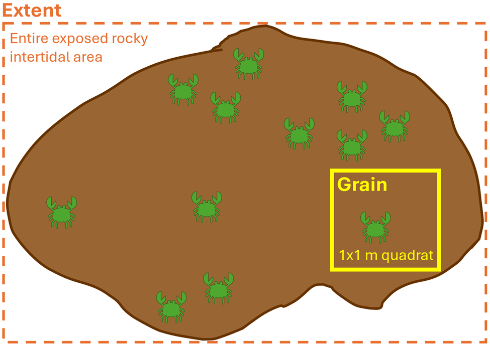
Observing and describing predator-prey relationships is complex due to the scale-dependent nature of these relationships (Levin, 1992). Each chapter of my dissertation considered krill, a globally-important prey type, from the perspective of baleen whales, which are krill predators. Chapter 2 used a comparative analysis to identify the optimal spatial scale at which to observe baleen whale-krill relationships on the Northern California Current (NCC) foraging grounds. We found correlations at a 5 km scale to be strongest, which can provide a useful starting point for further studies in the NCC and other systems. Chapter 3 used this spatial scale to compare several aspects of krill prey quality and quantity as predictors of humpback whale (Megaptera novaeangliae) distributions in the NCC. The best performing metric was a species, season, and spatially informed krill swarm biomass variable – yet the comparable performance of a simple acoustic abundance metric indicated that it can act as a reliable proxy for biomass. This finding may be advantageous for future research, as measuring the acoustic proxy is less computationally intensive and relies on fewer datastreams. Interestingly, one of this study’s best-performing models was based on only the proportion of Thysanoessa spinifera in krill swarms, which is also a highly accessible variable due to effective krill species distribution modeling in the NCC (Derville et al., 2024). Integrating the acoustic abundance proxy and krill species distribution predictions, two relatively simple metrics, could support predictions of humpback whale distributions in the NCC and inform whale-prey research in other ecosystems.

Figure 2. Collecting samples of individual krill gave us the opportunity to learn about their quality as prey for whales in the Northern California Current. Photo: Courtney Flatt

Studies relating predator foraging to prey characteristics often rely on metrics such as prey biomass or energy density (Schrimpf et al., 2012; Savoca et al., 2021; Cade et al., 2022), but the tendency of krill to form aggregations introduces dimensionality to krill prey quality. Chapter 4 showed that elements of krill swarm structure (particularly depth, proportion of T. spinifera, and metrics describing how krill occupy space within swarms) may be mechanistic drivers of variable blue, fin and humpback whale distribution patterns on the NCC foraging grounds. These findings suggest that krill swarm characteristics may be important links between baleen whales and the foraging environment. Swarm characteristics may be considered a component of krill prey quality for baleen whales, and future research could illuminate direct causal relationships between oceanographic conditions, krill swarming responses, and niche expression in baleen whale predators. 

The relationships between baleen whale distributions and krill quantity and quality explored in the first chapters of my dissertation may also shed light on other aspects of baleen whale ecology. The final chapter considers overwintering trends in global baleen whale populations, and examines the wintertime Western Antarctic Peninsula (WAP) as a case study. Extended humpback whale presence on the WAP feeding grounds may be driven by the profitable feeding areas and elevated energy content of krill during the winter months, and may reflect the high energetic needs of certain demographic subgroups (e.g. lactating females, juveniles). Wintertime humpback whale presence may also reflect adaptation to multifaceted competitive pressure on krill resources that are declining due to climate change (Atkinson et al., 2019), including consumption by growing baleen whale populations (Johnston et al., 2011) and a fishery whose catch limits may be impacting krill predators (Watters et al., 2020; Savoca et al., 2024). This work demonstrates how investigating prey quality during the winter months can contextualize baleen whale overwintering on the foraging grounds. It also provides a meaningful violation of the canonical baleen whale migration paradigm central to marine mammal science, which may lessen the efficacy of whale monitoring programs and management policies. 

Figure 3. We were surprised to see humpback whales like this one in Antarctica during the winter months — which raised a number of questions about overwintering of baleen whales on foraging grounds around the world. Photo: Giulia Wood

Management efforts that aim to mitigate risk to whales often hinge on predictive modeling of whale distributions. Species distribution models (SDMs) can provide managers with spatially and temporally explicit predictions of protected species occurrences (Wikgren et al., 2014; Santora et al., 2020), but species distributions in rapidly changing ecosystems are difficult to predict (Muhling et al., 2020). Findings from this dissertation may inform modeling efforts by suggesting meaningful predictor variables for SDMs, such as krill species on the NCC foraging grounds and swarm energy density at the WAP. This work also speaks to meaningful spatial scales for analyzing predator-prey relationships (i.e., 5 km), and relevant elements of temporal variability (e.g., seasonal cycles of krill energy density).

Just as marine predator-prey relationships are shaped by ocean processes, they likewise have consequences for those processes. For example, krill and other zooplankton are capable of generating large-scale mixing that can overcome stratification of water masses and alter water column structure (Noss and Lorke, 2014). Baleen whales influence global carbon cycles due to the huge amount of prey they consume (Savoca et al., 2021; Pearson et al., 2023) and transport important nutrients along the “great whale conveyer belt” during their vast migrations (Roman et al., 2025). Baleen whales seek krill as an essential prey resource on foraging grounds around the globe, and the impact of this trophic interaction scales up, with implications for ecosystem functioning and management. Continued research into the spatiotemporally dynamic relationships between krill and baleen whales improves our understanding of ocean functioning, and can improve our capacity to live as part of this system.

Loading

References

Atkinson, A., Hill, S. L., Pakhomov, E. A., Siegel, V., Reiss, C. S., Loeb, V. J., Steinberg, D. K., et al. 2019. Krill (Euphausia superba) distribution contracts southward during rapid regional warming. Nature Climate Change, 9: 142–147.

Cade, D. E., Kahane-Rapport, S. R., Wallis, B., Goldbogen, J. A., and Friedlaender, A. S. 2022. Evidence for Size-Selective Predation by Antarctic Humpback Whales. Frontiers in Marine Science, 9: 747788.

Derville, S., Fisher, J. L., Kaplan, R. L., Bernard, K. S., Phillips, E. M., and Torres, L. G. 2024. A predictive krill distribution model for Euphausia pacifica and Thysanoessa spinifera using scaled acoustic backscatter in the Northern California Current. Progress in Oceanography: 103388.

Fisher, J. L., Menkel, J., Copeman, L., Shaw, C. T., Feinberg, L. R., and Peterson, W. T. 2020. Comparison of condition metrics and lipid content between Euphausia pacifica and Thysanoessa spinifera in the northern California Current, USA. Progress in Oceanography, 188.

Fleming, A. H., Clark, C. T., Calambokidis, J., and Barlow, J. 2016. Humpback whale diets respond to variance in ocean climate and ecosystem conditions in the California Current. Glob Chang Biol, 22: 1214–24.

Hauser, D. D. W., Laidre, K. L., Stafford, K. M., Stern, H. L., Suydam, R. S., and Richard, P. R. 2017. Decadal shifts in autumn migration timing by Pacific Arctic beluga whales are related to delayed annual sea ice formation. Global Change Biology, 23: 2206–2217.

Johnston, S. J., Zerbini, A. N., and Butterworth, D. S. 2011. A Bayesian approach to assess the status of Southern Hemipshere humpback whales (Megaptera novaeangliae) with an application to Breeding Stock G. J. Cetacean Res. Manage.: 309–317. International Whaling Commission.

Lawrence, J. M. 1976. Patterns of Lipid Storage in Post-Metamorphic Marine Invertebrates. American Zoologist, 16: 747–762. Oxford University Press (OUP).

Levin, S. A. 1992. The Problem of Pattern and Scale in Ecology: The Robert H. MacArthur Award Lecture. Ecology, 73: 1943–1967.

McCabe, R. M., Hickey, B. M., Kudela, R. M., Lefebvre, K. A., Adams, N. G., Bill, B. D., Gulland, F. M., et al. 2016. An unprecedented coastwide toxic algal bloom linked to anomalous ocean conditions. Geophys Res Lett, 43: 10366–10376.

Muhling, B. A., Brodie, S., Smith, J. A., Tommasi, D., Gaitan, C. F., Hazen, E. L., Jacox, M. G., et al. 2020. Predictability of Species Distributions Deteriorates Under Novel Environmental Conditions in the California Current System. Frontiers in Marine Science, 7.

Noss, C., and Lorke, A. 2014. Direct observation of biomixing by vertically migrating zooplankton. Limnology and Oceanography, 59: 724–732. Wiley.

Oestreich, W. 2022. Acoustic signature reveals blue whales tune life‐history transitions to oceanographic conditions. Functional Ecology. https://besjournals.onlinelibrary.wiley.com/doi/10.1111/1365-2435.14013 (Accessed 20 September 2024).

Pearson, H. C., Savoca, M. S., Costa, D. P., Lomas, M. W., Molina, R., Pershing, A. J., Smith, C. R., et al. 2023. Whales in the carbon cycle: can recovery remove carbon dioxide? Trends in Ecology & Evolution, 38: 238–249.

Perryman, W. L., Joyce, T., Weller, D. W., and Durban, J. W. 2021. Environmental factors influencing eastern North Pacific gray whale calf production 1994–2016. Marine Mammal Science, 37: 448–462. Wiley.

Roman, J., Abraham, A. J., Kiszka, J. J., Costa, D. P., Doughty, C. E., Friedlaender, A., Hückstädt, L. A., et al. 2025. Migrating baleen whales transport high-latitude nutrients to tropical and subtropical ecosystems. Nature Communications, 16: 2125. Nature Publishing Group.

Ryan, J. P., Benoit-Bird, K. J., Oestreich, W. K., Leary, P., Smith, K. B., Waluk, C. M., Cade, D. E., et al. 2022. Oceanic giants dance to atmospheric rhythms: Ephemeral wind-driven resource tracking by blue whales. Ecology Letters, 25: 2435–2447.

Santora, J. A., Mantua, N. J., Schroeder, I. D., Field, J. C., Hazen, E. L., Bograd, S. J., Sydeman, W. J., et al. 2020. Habitat compression and ecosystem shifts as potential links between marine heatwave and record whale entanglements. Nat Commun, 11: 536.

Savoca, M. S., Czapanskiy, M. F., Kahane-Rapport, S. R., Gough, W. T., Fahlbusch, J. A., Bierlich, K. C., Segre, P. S., et al. 2021. Baleen whale prey consumption based on high-resolution foraging measurements. Nature, 599: 85–90.

Savoca, M. S., Kumar, M., Sylvester, Z., Czapanskiy, M. F., Meyer, B., Goldbogen, J. A., and Brooks, C. M. 2024. Whale recovery and the emerging human-wildlife conflict over Antarctic krill. Nature Communications, 15: 7708. Nature Publishing Group.

Schrimpf, M., Parrish, J., and Pearson, S. 2012. Trade-offs in prey quality and quantity revealed through the behavioral compensation of breeding seabirds. Marine Ecology Progress Series, 460: 247–259.

Watters, G. M., Hinke, J. T., and Reiss, C. S. 2020. Long-term observations from Antarctica demonstrate that mismatched scales of fisheries management and predator-prey interaction lead to erroneous conclusions about precaution. Scientific Reports, 10: 2314.

Wikgren, B., Kite-Powell, H., and Kraus, S. 2014. Modeling the distribution of the North Atlantic right whale Eubalaena glacialis off coastal Maine by areal co-kriging. Endangered Species Research, 24: 21–31.

New GEMM Lab study indicates troubled times for PCFG gray whales

Dr. Enrico Pirotta (CREEM, University of St Andrews) and Dr. Leigh Torres (GEMM Lab, MMI, OSU)

The health of animals affects their ability to survive and reproduce, which, in turn, drives the dynamics of populations, including whether their abundance trends up or down. Thus, understanding the links between health and reproduction can help us evaluate the impact of human activities and climate change on wildlife, and effectively guide our management and conservation efforts. In long-lived species, such as whales, once a decline in population abundance is detected, it can be too late to reverse the trend, so early warning signals are needed to indicate how these populations are faring.

We worked on this complex issue in a study that was recently published in the Journal of Animal Ecology. In this paper, we developed a new statistical approach to link three key components of the health of a Pacific Coast Feeding Group (PCFG) gray whale (namely, its body size, body condition, and stress levels) to a female’s ability to give birth to a calf. We were able to inform these metrics of whale health using an eight-year dataset derived from the GRANITE project of aerial images from drones for measurements of body size and condition, and fecal samples for glucocorticoid hormone analysis as an indicator of stress. We combined these data with observations of females with or without calves throughout the PCFG range over our study period.

We found that for a female to successfully have a calf, she needs to be both large and fat, as these factors indicate if the female has enough energy stored to support reproduction that year (Fig. 1). Remarkably, we also found indication that females with particularly high stress hormone levels may not get pregnant in the first place, which is the first demonstration of a link between stress physiology and vital rates in a baleen whale, to our knowledge.

Figure 1. Taken from Pirotta et al. (2025), Fig. 5. Combined relationship of PCFG gray whale length and nutritional state (combination of body size and condition) in the previous year with calving probability, colored by whether the model estimated an individual to have calved or not at a given reproductive opportunity.

Our study’s findings are concerning given our previous research indicating that gray whales in this PCFG sub-group have been growing to shorter lengths over the last couple of decades (Pirotta et al. 2023), are thinner than animals in the broader Eastern North Pacific gray whale population (Torres et al, 2022), and show an increase in stress-related hormones when exposed to human activities (Lemos et al, 2022; Pirotta et al. 2023). Furthermore, in our recent study we also documented that there are fewer young individuals than expected for a growing or stable population (Fig. 2), which can be an indicator of a population in decline since there may not be many individuals entering the reproductive adult age groups. Altogether, our results act as early warning signals that the PCFG may be facing a possible population decline currently or in the near future.

Figure 2. Taken from Pirotta et al. (2025), Fig. 1. Age structure diagram for 139 PCFG gray whales in our dataset. Each bar represents the number of individuals of a given age in 2023, with the color indicating the proportion of individuals of that age for which age is known (vs. estimated from a minimum estimate following Pirotta, Bierlich, et al., 2024). The red line reports a smooth kernel density estimate of the distribution.

These findings are sobering news for Oregon residents and tourists who enjoy watching these whales along our coast every summer and fall. We have gotten to know many of these whales so well – like Scarlett, Equal, Clouds, Lunita, and Pacman, who you can meet on our IndividuWhale website – that we wonder how they will adapt and survive as their once reliable habitat and prey-base changes. We hope our work sparks collective and multifaceted efforts to reduce impacts on these unique PCFG whales, and that we can continue the GRANITE project for many more years to come to monitor these whales and learn from their response to change.

This work exemplifies the incredible value of long-term studies, interdisciplinary methods, and effective collaboration. Through many years of research on this gray whale group, we have collected detailed data on diverse aspects of their behavior, ecology and life history that are critical to understanding their response to disturbance and environmental change, which are both escalating in the study region. We are incredibly grateful to the following members of the PCFG Consortium for contributing sightings and calf observation data that supported this study: Jeff Jacobsen, Carrie Newell, NOAA Fisheries (Peter Mahoney and Jeff Harris), Cascadia Research Collective (Alie Perez), Department of Fisheries and Oceans, Canada (Thomas Doniol-Valcroze and Erin Foster), Mark Sawyer and Ashley Hoyland, Wendy Szaniszlo, Brian Gisborne, Era Horton.

Did you enjoy this blog? Want to learn more about marine life, research, and conservation? Subscribe to our blog and get a weekly alert when we make a new post! Just add your name into the subscribe box below!

Loading

References:

Lemos, Leila S., Joseph H. Haxel, Amy Olsen, Jonathan D. Burnett, Angela Smith, Todd E. Chandler, Sharon L. Nieukirk, Shawn E. Larson, Kathleen E. Hunt, and Leigh G. Torres. “Effects of Vessel Traffic and Ocean Noise on Gray Whale Stress Hormones.” Scientific Reports 12, no. 1 (2022): 18580. https://dx.doi.org/10.1038/s41598-022-14510-5.

Pirotta, Enrico, K. C. Bierlich, Leslie New, Lisa Hildebrand, Clara N. Bird, Alejandro Fernandez Ajó, and Leigh G. Torres. “Modeling Individual Growth Reveals Decreasing Gray Whale Body Length and Correlations with Ocean Climate Indices at Multiple Scales.” Global Change Biology 30, no. 6 (2024): e17366. https://doi.org/https://doi.org/10.1111/gcb.17366. https://onlinelibrary.wiley.com/doi/abs/10.1111/gcb.17366.

Pirotta, Enrico, Alejandro Fernandez Ajó, K. C. Bierlich, Clara N Bird, C Loren Buck, Samara M Haver, Joseph H Haxel, Lisa Hildebrand, Kathleen E Hunt, Leila S Lemos, Leslie New, and Leigh G Torres. “Assessing Variation in Faecal Glucocorticoid Concentrations in Gray Whales Exposed to Anthropogenic Stressors.” Conservation Physiology 11, no. 1 (2023). https://dx.doi.org/10.1093/conphys/coad082.

Torres, Leigh G., Clara N. Bird, Fabian Rodríguez-González, Fredrik Christiansen, Lars Bejder, Leila Lemos, Jorge Urban R, et al. “Range-Wide Comparison of Gray Whale Body Condition Reveals Contrasting Sub-Population Health Characteristics and Vulnerability to Environmental Change.” Frontiers in Marine Science 9 (2022). https://doi.org/10.3389/fmars.2022.867258. https://www.frontiersin.org/article/10.3389/fmars.2022.867258

The slow, but ever turning, cycles of science: a look under the hood of the scientific method

Dr. Clara Bird, Postdoctoral Scholar, OSU Department of Fisheries, Wildlife, and Conservation Sciences, GEMM Lab & LABIRINTO

Cycles can be found everywhere in nature and our lives. From tides and seasons to school years and art projects, we’re constantly experiencing cycles of varying scales. Spring on the Oregon coast brings several important cyclical events: more daylight, the oceanographic spring transition, and the return of our beloved gray whales – just to name a few. On my own personal scale, I’ve been thinking about the cycles we experience as scientists a lot lately, since I’ve recently transitioned out of graduate school and into my current position as a postdoctoral scholar.

Starting this new postdoc has been a bit jarring, as it’s felt like starting over. Even though I’m still working at the Marine Mammal Institute and still studying gray whales, I’ve been learning new skills, knowledge and theory, which pushes me to re-start the cycle of the scientific method, the process we follow in research (Figure 1). Broadly, we start by observing a system and asking a question about a potential pattern or event we see. We then come up with a hypothesis (or two or ten) to address our question(s). The next steps are to collect the data we need to answer our question(s) and test our hypotheses, analyze that data (i.e. run some statistical models), and draw some conclusions from the analysis results. While it seems quite linear, the process of data collection and analysis always leads to more questions than answers, and we inevitably start the cycle all over again.

Figure 1. Schematic depicting the scientific method

Throughout my scientific training I’ve gained experience in all these phases, but I’ve also learned just how many add-ons and do-overs there are in this process (Figure 2). Developing questions and hypotheses often requires a long and winding path through the literature, depending on how much you already know. These steps are often some of the first and biggest steps in graduate school. You need to learn as much as you can about the field and questions you are interested in, as this will inform what has already been done, where the knowledge gaps are, and the hypotheses you’re developing. For example, we often back up a hypothesis with references to studies that have answered our question in different systems. The learning curve is steep, and it’s important to not understate the work that goes into this phase. Early in my career, I remember hearing that “asking the good questions” is a critical skill for research. At the time that sounded like some vague, innate characteristic, and working to gain this ability felt ambiguous and overwhelming. I was absolutely wrong. Like most skills, knowing how to ask good questions is more about experience than intelligence. Here, experience is a combination of reading the literature and practice formulating questions based on the literature.

Figure 2. A more realistic version of the scientific method

Beyond this lesson, I also had to learn that what qualifies a question as “good” also depends on the funding source. In many research institutions, including those in the U.S., scientists are responsible for finding the funding to run their research projects. Funding a project includes salary for the scientists (e.g., professors, grad students, post docs), the cost of collecting and analyzing the data (e.g., travel, equipment, boat time), and the cost of publishing and sharing our findings (e.g., publication costs). The programs we solicit funding from often have their own priorities, so a big part of the research cycle is finding a funding source that is interested in the kinds of questions you want to ask and then adjusting your own questions and hypotheses to align with the funding source’s priorities and budget. The actual application includes writing a proposal where we (1) summarize all the background research justifying the novelty and value of the questions we want to ask and backing up our hypotheses and (2) describe how we plan on answering those questions. Funding is competitive and we typically apply multiple times before being successful. Furthermore, we often apply to multiple funding sources to support the same project. Since each source has its own focus, this ends up being an exercise in coming up with multiple ways to frame and justify a project.

Once we have funding (which can be years after the start of the cycle), we can finally start collecting, analyzing, and interpreting the data. But each of these steps has its own sub-cycles and complexities. Data collection can take years and involve all kinds of troubleshooting equipment issues, logistics, and methods. Depending on your question, data processing and analysis may involve developing your own method. For example, our lab asks a lot of questions about the morphology and body condition of whales. But before we could answer those questions, we first had to work out the best way to accurately measure whales from drone imagery while accounting for measurement uncertainty (read more here). This separate cycle of method development involved so many sub-projects and new software tools that Dr. KC Bierlich now leads the Marine Mammal Institute’s Center of Drone Excellence (CODEX).

Data analysis and interpretation brings us back to the literature review part of the cycle. But now we are looking for examples of how similar data have been analyzed previously and for studies to which we can compare our results. Then, after testing out different models and triple checking our analysis, we’re finally ready to share our findings. We share our results through conference presentations, publications (after the peer review cycle), outreach talks, and press releases that lead to media pieces and interviews.

In addition to the excitement of sharing our findings with the world, we’re simultaneously hyper-aware of all the caveats and limitations of our work. We’re always left with a long list of follow-up questions, thus starting the cycle again. From a zoomed-out perspective these results can form a clean, linear story. But zooming in reveals the reality of years and years of multiple overlapping cycles that have had to pass roadblocks and restart countless times. For example, after nine years for research, the GRANITE project has produced an impressive suite of results addressing questions related to Pacific Coast Feeding Group gray whale morphology, health, hormones, space use, and behavior. It took years of data collection, proposal writing, training, and multiple researchers working through their own project cycles to get here (and we’re not done).

Transitioning out of graduate school has meant expanding my scope of attention to multiple cycles running in parallel, re-starting the literature review process for new projects, and spending a lot more time in the proposal writing sub-cycle. While it’s felt overwhelming at times, I’ve also enjoyed digging into new topics and skills. It’s an interesting balance of experiencing the discomfort that comes with being a beginner while simultaneously drawing comfort from the knowledge that I’ve experienced this cycle before and know how to learn something new.

A consequence of learning the scientific process is growing accustomed to this cyclical nature. As scientists we know that it’s a slow process, that every result is just the start of a new cycle, and that future work building on a result may agree or disagree with the previous finding. But the way scientific findings are shared with the public doesn’t necessarily reflect the process. Catchy headlines and brief summaries often present findings as definitive and satisfying conclusions to a story. Behind those headlines are years of set up, data collection, analysis, and a suite of caveats that we want to dig into in the future. The results of any given study reflect our best current knowledge at that point in the cycle. By design, that knowledge will grow and change as we move forward.

Did you enjoy this blog? Want to learn more about marine life, research, and conservation? Subscribe to our blog and get a weekly alert when we make a new post! Just add your name into the subscribe box below!

Loading

The Hitchhiker’s Guide to the Gray Whale: Cetacean Cyamid Coverage Explained

By Natalie Chazal, PhD student, OSU Department of Fisheries, Wildlife, & Conservation Sciences, Geospatial Ecology of Marine Megafauna Lab

When most people think about monitoring the health of a 40-ton gray whale, they picture blubber thickness, dive patterns, or perhaps growth rates. But what if some of the most telling signs are found not in the whale’s bulk, but right on the surface–embedded in its skin, and even crawling across it?

As part of the GRANITE project, my research focuses on using a long-term photographic dataset (>347,000 photos from 10 years!) to evaluate epidermal indicators of stress and health in Pacific Coast Feeding Group (PCFG) gray whales (Eschrichtius robustus) foraging off the Oregon coast. My central questions ask:

  • Can we use features visible on the skin like epidermal diseases, lesion severity, scarring from orcas, boats, and fishing gear, and potentially cyamid loads as biomarkers of physiological stress or nutritional status?
  • How do these skin-based indicators correlate with environmental variables, prey availability, fecal hormones, and overall body condition?

By tracking these patterns across individuals and years, my goal is to understand how gray whales are responding to a changing ocean and whether their skin can tell us more about what’s under the surface.

What are cyamids?

Cyamids, more commonly known as “whale lice”, are small crustaceans that live exclusively on marine mammals. Despite their nickname, cyamids are not true lice—they’re actually amphipod ectoparasites, more closely related to beach hoppers than anything you’d find in your hair. For gray whales (Eschrichtius robustus), these tiny passengers are a constant presence throughout their lives.

Figure 1. Gray whale blow hole area covered in barnacles and cyamids. The circle inset shows a zoomed in area where you can see the orange cyamids aggregating near the more yellow barnacles.

Each whale can host thousands of cyamids at a time, with individuals often clustering in specific areas of the body that provide physical refuge from the currents: around the blowhole, in the crevices of flukes, along the rostrum, genital slits, and especially around wounds or skin irregularities (Figure 1). Unlike barnacles, which attach directly to the skin and remain stationary while they feed on nutrients in the passing water, cyamids grasp onto the whale’s body using claw-like appendages, feeding on sloughed skin and bodily fluids. This relationship is generally not thought to be harmful to the whale, but high cyamid loads can be indicative of poor health, injury, or compromised immune function.

There are several species of cyamids, and many are host-specific—meaning they’ve evolved alongside particular whale species. In gray whales, the most common is Cyamus scammoni, which specializes on gray whales and is rarely found elsewhere. Other species found on gray whales include Cyamus kessleri, and the rarer Cyamus ceti. Cyamids are transmitted primarily from mother to calf, which helps explain their host fidelity, but horizontal transmission (between unrelated individuals) may also occur during close contact which can explain some rare occurrences of cyamids that are found outside of their general host species. In fact, Cyamus ceti was only found once on gray whales in 1861 but is generally thought to be specific to bowhead whales, giving us potential insight into interspecies interactions (bowhead and gray whales can spatially overlap on Arctic foraging grounds).

Figure 2. Cyamus scammoni close up photographs of (A) aggregation, (B) juvenile stage, (C) dorsal side of an adult, and (D) ventral side of an adult showcasing the cyamids corkscrew shaped gills (Takeda et al. 2005)

Because cyamids are permanent residents of the whale’s skin, they offer a unique window into both individual whale life histories and broader ecological trends. Their location, abundance, and distribution can potentially inform us about wound healing, residency duration in foraging areas, and even stress or health status—which makes them an unexpectedly valuable focal point in drone and photograph-based monitoring efforts like in the GRANITE project.

Cyamid Life History

Cyamids are obligate ectoparasites, meaning they spend their entire life on a whale and cannot survive independently in the open ocean. Unlike free-swimming crustaceans, cyamids are permanently attached to the skin or embedded within crevices of the whale’s body, often clinging to roughened areas, scars, embedded barnacles, or calloused skin where they can anchor themselves more securely.

They begin life as tiny juveniles, hatching from eggs carried in the brood pouch of a female cyamid. Rather than undergoing a larval phase in the water column like many marine invertebrates, cyamids develop directly into miniature versions of adults and remain on the whale from birth. This direct development is essential because there’s no safe habitat for a larval cyamid in the open ocean: the host whale is both nursery and home.

Most transmission occurs from mother to calf during the close physical contact of early life. Calves born in the warm lagoons of Baja California, Mexico where gray whales calve and nurse during the winter inherit their cyamid colonies during nursing, rubbing, and swimming alongside their mothers. These early colonizers will multiply as the calf grows and can remain with the whale for years, forming the basis of a persistent, host-specific population.

For Cyamus scammoni specifically (our gray whale specific cyamid), adults will breed in the summer just before the southbound migration. Females will have around 1,000 eggs in their brood pouch, although only about a 60% are fertilized (Leung, 1976). These eggs will hatch in the fall while the gray whales take on their southbound migration but they will stay in the safety of the brood pouch for around 2 to 3 months. The juveniles will be released in the winter, when gray whales arrive in the Baja lagoons where they will then find shelter within the crevices of their host gray whale. Juveniles reach maturity during the northbound migration and will be a full-grown brood upon arrival to summer grounds. While the cycle takes about 8 months to complete, there are juveniles found along the gray whales year-round, leading us to believe that there is likely overlap between broods. For our less abundant Cyamus kessleri, the life cycle is very similar, but the juveniles reach maturity before the gray whales northbound migration to summer feeding grounds. Also, there are around 300 eggs in the Cyamus kessleri brood pouches that have a higher rate of fertilization (75-80%) than Cyamus scammoni (60%) (Leung, 1976)

In short, the life of a cyamid is fully bound to the life of a whale. Every migration, dive, foraging event, and scar the whale experiences becomes part of the cyamid’s environment. By studying them, we gain another lens through which to interpret the health, behavior, and ecology of gray whales on the Oregon Coast.

Uses in Cetacean Health Assessments

As we’ve established, cyamids have unique life histories as ectoparasites and may be valuable indicators in cetacean health assessments across multiple whale species. Because they often congregate around wounds, lesions, and areas of poor skin integrity, their presence and distribution can reveal important clues about a whale’s physical condition, injury history, and immune response. However, studies that have made these connections have variable results.

In species like North Atlantic right whales (Pettis et al. 2004, Pirotta et al. 2023), harbor porpoises (Lehnert et al. 2021), and gray whales (Raverty et al. 2024), researchers have used visual surveys and photographic analysis to quantify cyamid loads in living, stranded, and hunted whales. Researchers can score cyamid presence by identifying attachment sites (e.g. blowhole, scar, dorsal ridge) and estimating the relative coverage by using standardized reference images to maintain consistency. In these studies, whales with heavy cyamid coverage, especially in sensitive regions like the blowhole, mouthline, and genital area, often show signs of poor health or stress, such as emaciation, scarring from entanglement, or chronic skin conditions. Cyamid coverage is sometimes used alongside body condition indices and lesion scoring to build a more complete health profile (Pirotta et al. 2023). There are also studies that show no connections, or even positive connections between body condition and cyamid coverage (Von Duyke et al. 2016).

While cyamids are often associated with injured, inflamed, or otherwise damaged skin, there is no evidence that points towards cyamids directly damaging the skin themselves. However, more work needs to be done to assess their role in the healing processes. Additionally, it’s been noted that more work is needed on the role of cyamids and disease spread (Overstreet et al. 2009). For the PCFG, there is an iconic whale we call “Scarlett” (also known as “Scarback”) who has a large scar on the right side of her back that is highly identifiable due to the orange swarm of cyamids that are constantly surrounding the edges of the wound. She has managed to survive and thrive, producing many calves over the years, but questions remain: How are the cyamids affecting the healing process? Are they increasing or decreasing the risk of infection? How does the frequency of large injuries like this on whales contribute to the cyamid population over evolutionary time?

Figure 3. Right side of PCFG icon, “Scarlett” showing her massive scar covered with orange aggregations of cyamids.

Because whales are complex, highly mobile, long-lived creatures with a constant population of cyamid hitchhikers their skin condition is likely representative of specific to life history, phylogeography, and demographic traits of individuals. While we know that cyamids generally eat sloughed or damaged skin on the whale, what this behavior and symbiosis means for each whale’s individual physiology can be highly complex. Through our high-resolution drone and lateral imagery of the same individuals over time paired with other data sources, such as body condition and prey availability, cyamid scores can offer key insights into how environmental stressors and foraging success affect individual and population-level whale health.


These tiny crustaceans, clinging to the folds and scars of their hosts, might seem like background noise in a study focused on body condition or foraging ecology—but they’re far from incidental. In my research, I’ve come to see cyamids as part of the bigger story: silent indicators of stress, recovery, movement, and resilience. By pairing imagery of PCFG gray whale skin with data on prey availability and environmental conditions, I’m working to understand how foraging success and anthropogenic stressors (such as vessel traffic and entanglements) manifest not just in a whale’s body condition, but in the skin itself. The presence, distribution, and density of cyamids may offer yet another layer of insight into how gray whales are coping with changing ocean conditions. It’s a reminder that even the smallest details, like a patch of whale lice, can help us ask bigger questions about the health, resilience, and future of these cetaceans.

References

Callahan, C.M., n.d. MOLECULAR SYSTEMATICS AND POPULATION GENETICS OF WHALE LICE (AMPHIPODA: CYAMIDAE) LIVING ON GRAY WHALE ISLANDS.

Lehnert, K., IJsseldijk, L.L., Uy, M.L., Boyi, J.O., van Schalkwijk, L., Tollenaar, E.A.P., Gröne, A., Wohlsein, P., Siebert, U., 2021. Whale lice (Isocyamus deltobranchium & Isocyamus delphinii; Cyamidae) prevalence in odontocetes off the German and Dutch coasts – morphological and molecular characterization and health implications. International Journal for Parasitology: Parasites and Wildlife 15, 22–30. https://doi.org/10.1016/j.ijppaw.2021.02.015

Leung, Y., 1976. Life cycle of cyamus scammoni (amphipoda: cyamidae), ectoparasite of gray whale, with a remark on the associated species. Scientific Reports of the Whales Research Institute 28, 153–160.

Overstreet, R.M., Jovonovich, J., Ma, H., 2009. Parasitic crustaceans as vectors of viruses, with an emphasis on three penaeid viruses. Integrative and Comparative Biology 49, 127–141. https://doi.org/10.1093/icb/icp033

Pettis, H.M., Rolland, R.M., Hamilton, P.K., Brault, S., Knowlton, A.R., Kraus, S.D., 2004. Visual health assessment of North Atlantic right whales (Eubalaena glacialis) using photographs. Can. J. Zool. 82, 8–19. https://doi.org/10.1139/z03-207

Pirotta, E., Schick, R.S., Hamilton, P.K., Harris, C.M., Hewitt, J., Knowlton, A.R., Kraus, S.D., Meyer-Gutbrod, E., Moore, M.J., Pettis, H.M., Photopoulou, T., Rolland, R.M., Tyack, P.L., Thomas, L., 2023. Estimating the effects of stressors on the health, survival and reproduction of a critically endangered, long-lived species. Oikos 2023, e09801. https://doi.org/10.1111/oik.09801

Raverty, S., Duignan, P., Greig, D., Huggins, J.L., Huntington, K.B., Garner, M., Calambokidis, J., Cottrell, P., Danil, K., D’Alessandro, D., Duffield, D., Flannery, M., Gulland, F.M., Halaska, B., Lambourn, D.M., Lehnhart, T., Urbán R., J., Rowles, T., Rice, J., Savage, K., Wilkinson, K., Greenman, J., Viezbicke, J., Cottrell, B., Goley, P.D., Martinez, M., Fauquier, D., 2024. Gray whale (Eschrichtius robustus) post-mortem findings from December 2018 through 2021 during the Unusual Mortality Event in the Eastern North Pacific. PLoS One 19, e0295861. https://doi.org/10.1371/journal.pone.0295861

Stimmelmayr, R., Gulland, F.M.D., 2020. Gray Whale (Eschrichtius robustus) Health and Disease: Review and Future Directions. Front. Mar. Sci. 7. https://doi.org/10.3389/fmars.2020.588820

Takeda, M., Ogino, M., n.d. Record of a Whale Louse, Cyamus scammoni Dall (Crustacea: Amphipoda: Cyamidae), from the Gray Whale Strayed into Tokyo Bay, the Pacific Coast of Japan.

Von Duyke, A.L., Stimmelmayr, R., Sheffield, G., Sformo, T., Suydam, R., Givens, G.H., George, J.C., 2016. Prevalence and Abundance of Cyamid “Whale Lice” (Cyamus ceti) on Subsistence Harvested Bowhead Whales (Balaena mysticetus). Arctic 69, 331–340.

Würsig, B., Thewissen, J.G.M., Kovacs, K.M., 2017. Encyclopedia of Marine Mammals. Elsevier Science & Technology, Chantilly, UNITED STATES.

The whale’s scale: Emphasizing the scale of process, not the scale of observation

By Lisa Hildebrand, PhD candidate, OSU Department of Fisheries, Wildlife, & Conservation Sciences, Geospatial Ecology of Marine Megafauna Lab

Baleen whales must navigate a seemingly featureless world to locate the resources they need to survive. The task of finding prey to feed on in the vast seascapes relies on the use of several sensory modalities that operate at different scales (Torres 2017; Figure 1). For example, baleen whale vision is believed to be rather limited, with the ability to see objects about 10-100 meters away. Yet, baleen whale somatosensory perception of oceanographic stimuli is thought to be on the order of 100-1000s kilometers. This diversity in sensory ability has led scientists to believe that whales, in fact all animals, perceive cues and make decisions at several scales. As ecologists, we endeavor to understand why and when animals are found (or not found) in certain locations as this knowledge allows us to better manage and conserve animal populations. With this information we can aim to minimize potential anthropogenic disturbance and protect important resource areas, such as foraging or nursing grounds. In order to accomplish this goal, we ourselves must conduct studies and test hypotheses at several scales (Levin 1992; Hobbs 2003). As someone who tackles spatial foraging ecology questions, I am particularly interested in understanding whale behavior and movement in the context of feeding. Since accurately measuring predator and prey distribution at the same scales can be challenging, we often resort to environmental variables to serve as proxies for prey, whereby we look for correlations between environmental variables and whales to understand and predict the distribution of our population. 

Figure 1. Schematic of hypothetical interchange of sensory modalities used by baleen whales to locate prey at variable scales. X-axis represents log distance to prey from micro (left) to macro (right). Y-axis represents the relative use of each sensory modality between 0 (no contribution) to 10 (highest contribution). Each line and color represent a different sensory modality. Figure taken and caption adapted from Torres 2017.

What do I mean when I use the word ‘scale’? The term scale is typically explained by two components: grain and extent (Wiens 1989). The grain is the finest resolution measured; in other words, how detailed we are measuring. The extent is the overall coverage of what we are measuring. These components can be applied to both spatial scale and temporal scale. For example, spatially, if we were using a 1×1 meter sampling quadrat to count the number of crabs on a rocky shore, then our grain would be the 1 m2 quadrat and the extent would be the entire exposed rocky intertidal area that we are surveying (Figure 2). Temporally, if we placed a temperature logger at the mouth of Yaquina Bay that took a temperature recording every minute for two years, then our grain would be one minute and the extent would be two years. So, when designing a study, it is imperative for us to decide on the spatiotemporal scales of the ecological questions we are asking and the hypotheses we are testing, as it will inform what data we need to collect. When making this decision, it is important to think about the scale at which the ecological process happens, as opposed to the scale at which we can observe the process (Levin 1992). In other words, we need to think from the perspective of our study species, as opposed to from our own human perspective. Making informed and ecologically reasonable decisions regarding the choice of scale relies on having prior knowledge of an animal’s biology, such as knowing that baleen whales might see a prey patch that is 50 meters away, but it may also somatosensorily perceive an oceanic front where zooplankton prey aggregate from 500 kilometers away.

Figure 2. Schematic of spatial scale where the extent (depicted by dashed orange box) is the entire exposed rocky intertidal area being surveyed and the grain (solid yellow box) is the 1×1 m quadrat being used to count crabs.

There is a wealth of studies that have explored space use patterns of wildlife relative to environmental variables to better understand foraging behavior. I want to share a couple from the marine mammal realm with you that I find particularly fascinating. In their 2018 study, González García and colleagues used opportunistic sightings of blue whales around the Azorean islands of Portugal and modeled their distribution patterns relative to physiographic and oceanographic variables summarized at different spatial (fine [1-10 km] and meso [10-100 km]) and temporal (daily, weekly, monthly) scales. The two variables that were most correlated with blue whale occurrence was distance from the coast and eddy kinetic energy (a measure of mesoscale variability of ocean dynamics). Both of these variables were interestingly found to be scale invariant, meaning that no matter which spatial and temporal scale was investigated, the relationship between blue whales and these two variables stayed the same; blue whale occurrence increased with increasing distance from the coast and was maximal at an eddy kinetic energy value of 0.007 cm2/s2 (Figure 3).

Figure 3. Functional response curves between presence of Azorean blue whales and distance to the coast (panel 1 on left) and eddy kinetic energy (panel 2 on right). The top row of each panel represents the low spatial scale and the bottom row represents the high spatial scale. Each column represents a different temporal scale (from left to right: daily, weekly, monthly). Note that the general shape of the relationship remains similar across all spatiotemporal scales and that the peak of the curves tend to occur at the same values for distance to coast and eddy kinetic energy across all scales. Figures taken from González García et al. 2018.

However, not all studies find scale invariant relationships. For example, Cotté and co-authors (2009) found that habitat use of Mediterranean fin whales was very much scale dependent. At a large scale (700-1,000 km and annual), fin whales were more densely aggregated during the summer in the Western Mediterranean where there was consistently colder water than in the winter. However, at a meso scale (20-100 km and weekly-monthly), fin whale densities were highest in areas where there were steep changes in temperature, as opposed to consistently cold temperatures. The authors explain that these differences in fin whale density and temperature at different scales are likely due to whale movement being driven by annually persistent prey abundance at the large scale, but at the meso scale, where prey aggregations are less predictable, the fin whales’ distribution becomes more driven by areas of physical ocean mixing.

As I investigate the environmental drivers of individual gray whale space use using our 8-year GRANITE (Gray whale Response to Ambient Noise Informed by Technology and Ecology) dataset, these studies (and many more) are at the top of my mind to interpret the patterns we are detecting. Our goal is to quantify and describe what environmental conditions (1) lead to a higher probability of a gray whale being seen in our central Oregon coast study area (~70 km) at a daily scale, and (2) influence space use patterns (activity range, residency, activity center) of different individual whales at annual scales. Our results show both consistency and variation in the environmental drivers of gray whales across these scales, leading me to deeply consider how gray whales make decisions at different points in their lives, based on information gained through various senses, to maximize their chances of capturing food. Previous work from the GEMM Lab on the relationships between gray whales and prey, at both fine (read more here) and large (read more here) scales have guided my work by providing specific hypotheses regarding environmental variables and lag times for me to test. Investigating the environmental drivers of animal space use and behavior is exciting work as it reveals that no single environmental variable determines animal distribution, but rather that multiple processes are happening concomitantly that animals respond to at different scales continually. It is only by studying animal space use patterns across spatiotemporal scales that we can begin to understand their complex decision-making patterns.

Did you enjoy this blog? Want to learn more about marine life, research, and conservation? Subscribe to our blog below and get a monthly message when we post a new blog. Just add your name and email into the subscribe box below.

Loading

References

Cotté, C., Guinet, C., Taupier-Letage, I., Mate, B., & Petiau, E. (2009). Scale-dependent habitat use by a large free-ranging predator, the Mediterranean fin whale. Deep Sea Research Part I: Oceanographic Research Papers56(5), 801-811.

González García, L., Pierce, G. J., Autret, E., & Torres-Palenzuela, J. M. (2018). Multi-scale habitat preference analyses for Azorean blue whales. PLoS One13(9), e0201786.

Hobbs, N. T. (2003). Challenges and opportunities in integrating ecological knowledge across scales. Forest Ecology and Management181(1-2), 223-238.

Levin, S. A. (1992). The problem of pattern and scale in ecology: the Robert H. MacArthur award lecture. Ecology73(6), 1943-1967.

Torres, L. G. (2017). A sense of scale: Foraging cetaceans’ use of scale‐dependent multimodal sensory systems. Marine Mammal Science33(4), 1170-1193.

Wiens, J. A. (1989). Spatial scaling in ecology. Functional ecology3(4), 385-397.

The blues are back in town: recap of the SAPPHIRE 2025 field season

By Dr. Dawn Barlow & Dr. Leigh Torres, OSU Department of Fisheries, Wildlife, and Conservation Sciences, Geospatial Ecology of Marine Megafauna Lab

As the sun set on February 16th, the R/V Star Keys pulled into Wellington Harbour, marking the end of the 2025 SAPPHIRE field season. The crew and science team returned to shore after a packed, productive, and successful three weeks at sea studying the impacts of environmental change on blue whales and krill in the South Taranaki Bight, Aotearoa New Zealand.

A blue whale comes up for air in the South Taranaki Bight.

In stark contrast to the 2024 field season, which featured dense and seemingly endless layers of gelatinous salps in the water and no krill or blue whales in the South Taranaki Bight, the 2025 field season was filled with blue whales and krill. In our three weeks aboard our research vessel Star Keys this year, we observed 66 blue whales, most of which were lunge feeding at the surface on dense patches of krill. We also collected krill for on-board respiration experiments and to be frozen to measure their lengths, weights, and caloric content. We recovered two hydrophones that recorded blue whale calls for the past year, and replaced them with two more. We collected identification photos, skin and blubber tissue samples for genetic and hormone analysis, and flew drones over almost all whales we encountered to measure body condition and morphology. We conducted water column profiles to measure the oceanography of the region, and mapped the prey field as we surveyed using a scientific echosounder.

Map of our survey effort (gray tracklines), blue whale sightings (red circles), and hydrophone locations (purple stars).

Around the world, we are currently bearing witness to environmental change. Our survey last year in 2024 was a reminder of the challenges these blue whales face to survive and thrive in an increasingly unpredictable ocean. This year was a poignant example of the vibrant marine life that exists here in the South Taranaki Bight when ocean conditions align more closely with what is expected, and of the incredible resilience of these animals as they navigate changing waters. These contrasting conditions over multiple years are key to our understanding as we study the impacts of climate change on krill and blue whales through the SAPPHIRE project.

Drone image of a blue whale coming to the surface.

The fieldwork we do to collect these data is motivated by scientific questions, management needs, and fascination with this ecosystem. But ultimately, what makes fieldwork possible and memorable is the people. We are deeply grateful for the many partners on the SAPPHIRE project. The 2025 science team was made up of Leigh Torres, Dawn Barlow, KC Bierlich, Kim Bernard (Oregon State University), Mike Ogle, and Ros Cole (Department of Conservation). The outstanding crew of the R/V Star Keys (Western Work Boats), Josh Fowden, Dave Futter, and Jordy Maiden-Drum, kept us safe, sailing, fed, and happy for three intense weeks. We are also grateful for our shore support, including our colleagues at Cornell University’s Yang Center for Conservation Bioacoustics, NIWA, the Marine Mammal Institute at Oregon State University, and the University of Auckland. Importantly, we deeply appreciate our many stakeholders who help us share, learn, and make our findings meaningful, including the Department of Conservation, the people of Aotearoa, and iwi across our study region, especially Ngāruahine who hosted us at the Rangatapu Marae for a profound hui with a powerful pōwhiri and critical wānanga of knowledge sharing.

Drone image of a blue whale mom and calf pair.

Now the next phase of the work begins. We have many terabytes of data to process, analyze, interpret, and share. We will certainly have our hands full. But while we are at our computers back in Oregon, we will be holding the memories of this field season close: The brilliant turquoise glow of a blue whale just below the surface, the sound of the deep exhalation as the whale comes up for air, and the awe of looking into a blue whale’s eye as it engulfs a dense swarm of krill; The golden sunset lighting and moon rise over Cape Farewell, and Mount Taranaki towering over the blue waters of the South Taranaki Bight; The giddy exclamations or silent awe of those of us privileged to spend time in these waters observing these animals, and the visions that linger just behind our eyelids as we fell into an exhausted sleep. We will see what the next year holds for the SAPPHIRE team and the blue whales and krill of the South Taranaki Bight.

Did you enjoy this blog? Want to learn more about marine life, research, and conservation? Subscribe to our blog and get a weekly alert when we make a new post! Just add your name into the subscribe box below!

Loading

New publication shows humpback whale distribution in the Northern California Current is related to krill swarm biomass, energetic density, and species composition

By Rachel Kaplan, PhD candidate, Oregon State University College of Earth, Ocean, and Atmospheric Sciences and Department of Fisheries, Wildlife, and Conservation Sciences, Geospatial Ecology of Marine Megafauna Lab

What does a whale look for at mealtime? Is it a lot of food, its quality, or the type of food? An improved understanding of what makes krill swarms, an important prey item, appetizing for humpback whales can help us anticipate where and when we will see them in our ocean backyard, the Northern California Current (NCC) foraging grounds. In a new paper, we found that humpback whale presence in the NCC is tied to several different metrics of krill swarm quality and quantity, particularly species composition (what types of krill are in the swarm), energetic density (the caloric richness of the average mouthful), and biomass (how much krill is in the swarm). Interestingly, relationships between humpback whales and these krill swarm quality metrics are variable in time and space, dependent on whether the whale is foraging on or off the continental shelf and if it is early or late in the foraging season.

This study required a special, fine-scale dataset of simultaneous observations of krill and whales at sea. While GEMM Lab members conducted marine mammal surveys, we simultaneously observed the prey that whales had access to, using active acoustics (essentially a fancy fish finder) to profile the water column and net tows to collect krill. When we put all these data streams together, we found that increases in biomass, energetic density, and the amount of a particular species, Thysanoessa spinifera, in a krill swarm were positively related to humpback whale presence. These results suggest that humpback whales balance multiple prey quality factors to select feeding areas that offer both plentiful and high-quality krill.

Figure 1. Top photo: Marine mammal observers Clara Bird (left) and Dawn Barlow (right) collect humpback whale distribution data. Bottom photo: At the same time, Talia Davis (left) and Rachel Kaplan (right) collect krill samples.

Species composition

Euphausia pacifica and T. spinifera are the two most common krill species in the NCC region, and other research has shown that many krill foragers, including blue whales, seabirds, and fish, preferentially consume T. spinifera. Although this pickiness is well-warranted – individual T. spinifera tend to be larger than E. pacifica and much higher in calories during the late foraging season – targeting this juicy prey item could place humpback whales in competition with these other species, which may make it harder for them to find a square meal. Nevertheless, we found positive relationships between the proportion of T. spinifera in a krill swarm and humpback whale presence, suggesting humpback whales do in fact preferentially prey upon T. spinifera, particularly during the late foraging season (about July-November).

Energetic density

Humpback whales’ preference for T. spinifera during the late foraging season may be due to its higher caloric content. Although the two krill species offer a similar number of calories early in the foraging season,we found that the energetic density of T. spinifera was elevated during the late foraging season, after productive upwelling conditions have revved up the food web over several months. Krill swarm energetic density had a positive effect on humpback whale occurrence, particularly in the late season when T. spinifera and E. pacifica have significantly different caloric contents. Interestingly, this positive relationship was not present onshore during the early season, when the two krill species have similar caloric contents.

Figure 2. In terms of caloric content, Thysanoessa spinifera krill like this one are the winners in the NCC region! They pack on the milligrams through the productive summer season, making them advantageous prey for hungry whales.

Humpback whales also target forage fish on the continental shelf that have higher energetic densities than krill, indicating that whales may selectively forage on fish – even though it is more energetically expensive to capture them. Variation in seasonal and spatial relationships with krill swarm energetic density may explain why humpback whales prey-switch, selecting prey based on availability and quality. As flexible foragers, humpback whales can consistently target higher-quality swarms that offer more energy per lunge.

Biomass

Biomass, or the total amount of krill in a swarm, was the single best predictor of humpback whale presence that we tested. This result emphasizes the importance of large krill swarms in explaining where humpback whales forage. We found that krill swarm biomass tended to be higher offshore, where swarms were also located deeper in the water column. During the late season offshore, krill quality (elevated due to higher late season caloric contents) together with quantity (higher offshore biomass) may make these offshore swarms the most favorable for foraging whales, despite being deeper.

Figure 3. When humpback whales “fluke,” as seen in this picture, it may indicate the beginning of a foraging dive to capture prey.

Future food webs

Environmental conditions are changing in the NCC, with events like marine heatwaves and strong El Niño events shifting food webs. E. pacifica and T. spinifera may respond to climate change differently based on their life history strategies. Distributional shifts, such as the disappearance of T. spinifera from the NCC during the 2014–2015 “Blob” marine heatwave that transformed the northeast Pacific Ocean, could diminish or entirely remove this key prey item. As a result of such climate and environmental changes, humpback whales may encounter lower quality prey and/or shifts in prey distribution that could make it harder for them to find a meal. In changing oceans, better understanding krill prey quality for humpback whales will shape improved tools for conservation management.

Loading

References

Chenoweth, E., Boswell, K., Friedlaender, A., McPhee, M., Burrows, J., Heintz, R., and Straley, J. 2021. Confronting assumptions about prey selection by lunge‐feeding whales using a process‐based model. Funct. Ecol., 35.

Croll, D., Marinovic, B., Benson, S., Chavez, F., Black, N., Ternullo, R., and Tershy, B. 2005. From wind to whales: trophic links in a coastal upwelling system. Mar. Ecol. Prog. Ser., 289: 117–130.

Derville, S., Buell, T. V., Corbett, K. C., Hayslip, C., and Torres, L. G. 2023. Exposure of whales to entanglement risk in Dungeness crab fishing gear in Oregon, USA, reveals distinctive spatio-temporal and climatic patterns. Biol. Conserv., 281: 109989.

Fiedler, P. C., Reilly, S. B., Hewitt, R. P., Demer, D., Philbrick, V. A., Smith, S., Armstrong, W., et al. 1998. Blue whale habitat and prey in the California Channel Islands. Deep Sea Res. Part II, 45: 1781–1801.

Fisher, J. L., Menkel, J., Copeman, L., Shaw, C. T., Feinberg, L. R., and Peterson, W. T. 2020. Comparison of condition metrics and lipid content between Euphausia pacifica and Thysanoessa spinifera in the northern California Current, USA. Prog. Oceanogr., 188.

Murdoch, W. W. 1969. Switching in General Predators: Experiments on Predator Specificity and Stability of Prey Populations. Ecol. Monog., 39: 335–354.

Nickels, C. F., Sala, L. M., and Ohman, M. D. 2018. The morphology of euphausiid mandibles used to assess selective predation by blue whales in the southern sector of the California Current System. J. Crustacean Biol., 38: 563–573.

Price, S. E., Savoca, M. S., Kumar, M., Czapanskiy, M. F., McDermott, D., Litvin, S. Y., Cade, D. E., et al. 2024. Energy densities of key prey species in the California Current Ecosystem. Front. Mar. Sci., 10: 1345525.

Robertson, R. R., and Bjorkstedt, E. P. 2020. Climate-driven variability in Euphausia pacifica size distributions off northern California. Prog. Oceanogr., 188.

Santora, J. A., Mantua, N. J., Schroeder, I. D., Field, J. C., Hazen, E. L., Bograd, S. J., Sydeman, W. J., et al. 2020. Habitat compression and ecosystem shifts as potential links between marine heatwave and record whale entanglements. Nat Commun, 11: 536.

Spitz, J., Trites, A. W., Becquet, V., Brind’Amour, A., Cherel, Y., Galois, R., and Ridoux, V. 2012. Cost of Living Dictates what Whales, Dolphins and Porpoises Eat: The Importance of Prey Quality on Predator Foraging Strategies. PLoS ONE, 7: e50096.

Tanasichuk, R. 1998a. Interannual variations in the population biology and productivity of Thysanoessa spinifera in Barkley Sound, Canada, with special reference to the 1992 and 1993 warm ocean years. Mar. Ecol. Prog. Ser., 173: 181–195.

Videsen, S. K. A., Simon, M., Christiansen, F., Friedlaender, A., Goldbogen, J., Malte, H., Segre, P., et al. 2023. Cheap gulp foraging of a giga-predator enables efficient exploitation of sparse prey. Sci. Adv., 9: eade3889.

Weber, E. D., Auth, T. D., Baumann-Pickering, S., Baumgartner, T. R., Bjorkstedt, E. P., Bograd, S. J., Burke, B. J., et al. 2021. State of the California Current 2019–2020: Back to the Future With Marine Heatwaves? Front. Mar. Sci., 8.


Demystifying AI: a brief overview of Image-Pre-Processing and a Machine Learning Workflow

Celest Sorrentino, MSc student, OSU Dept of Fisheries, Wildlife and Conservation Sciences, GEMM Lab

The first memory I have of A.I. (Artificial Intelligence) stems from one of my favorite movies growing up: I, Robot (2004). Shifting focus from the sci-fi thriller plot, the distinguished notion of a machine integrating into normal everyday life to perform human tasks, such as converse and automate labor, sparks intrigue. In 2014, my own realization of sci-fi fantasy turned reality initiated with the advertisements of self-driving cars by TESLA. But how does one go from a standard tool, like a vehicle, to an automated machine?

Fig 1: Tesla Self-Driving car, image by Bloomberg.com

For my first thesis chapter, I am applying a machine learning model to our lab’s drone video dataset to understand whale mother-calf associations, which is in continuation of my previous internship in 2022. A.I. has absolutely skyrocketed in marine science and hundreds of papers have confirmed the advantage in using machine learning models, such as in species abundance estimates (Boulent et al 2023), whale morphometrics (Bierlich et al 2024), and even animal tracking (Periera et al 2022). Specifically, Dr. KC Bierlich recently led a publication on an incredible A.I. model that can extract still images from drone footage to be subsequently used for body morphometric analysis. Earlier this year my lab mate Nat wrote an insightful blog introducing the history of A.I. and how she uses A.I. for image segmentation to quantify mysid swarms. For those of us who study animal behavior and utilize video-based tools for observation, A.I. is a sweet treat we’ve been craving to speed up and improve our analyses —but where do we start?

With a Venn Diagram and definitions of course!

Figure 1: Venn diagram demonstrating the relationships of 4 subsets of AI (Machine learning, Deep-learning, Computer Vision, and Natural Language Processing) and how they relate to one another.

Good terms to know:

Artificial Intelligence: a machine/model built to mimic human intelligence.

Machine Learning: a subset of A.I. that uses statistical algorithms to recognize patterns and form predictions, usually requiring human intervention for correction.

Deep-learning: a specific form of machine learning that is meant to mimic human neural networks through artificial neural networks (ANN) by recognizing hierarchal patterns with minimal to no human-intervention to correct.

Computer Vision: a type of machine learning that enables a machine/model to gather and retain information from images, video, etc.

Natural Language Processing: a subset of machine learning in which a machine/model to identify, understand, and create text and speech.

(Still a bit confused? A great example of the difference between machine learning and deep-learning can be found here)

So, you have a dataset, what’s the pipeline?

Figure 2: How to go from your research question and use your dataset to using an A.I. model.

First, we must consider what type of data we have and our question. In fact, you might find these two questions are complimentary: What type of questions does our dataset inspire and/or what type of dataset is needed to answer our question?

Responses to these questions can guide whether A.I. is beneficial to invest in and which type to pursue. In my case, we have an imagery dataset (i.e., drone videos) and our question explores the relationship of mom-calf proximity as an indicator of calf-independence. Therefore, a model that employs Computer Vision is a sensible decision because we need a model that extracts information from imagery. From that decision, I then selected SLEAP A.I. as the deep-learning model I’ll use to identify and track animals in video (Pereira et al 2022).

Figure 3: A broad schematic of the workflow utilizing a computer vision* model. As detailed above, a computer vision model is a machine learning model that uses images/videos as a dataset to retain information.

Why is image pre-processing important?

Image pre-processing is an essential step in “cleaning” the imagery data into a functional and insightful format for the machine learning model to extract information. Although tedious to some, I find this to be an exciting yet challenging step to push my ability to reframe my own perspective into another, a trait I believe all researchers share.

A few methods for image/video preprocessing include Resizing, Grayscaling, Noise Reduction, Normalization, Binarization, and Contrast enhancement. I found the following definitions and Python code by Maahi Patel to be incredibly concise and helpful. (Medium.com)

• Resizing: Resizing images to a uniform size is important for machine learning algorithms to function properly. We can use OpenCV’s resize() method to resize images.
• Grayscaling: Converting color images to grayscale can simplify your image data and reduce computational needs for some algorithms. The cvtColor() method can be used to convert RGB to grayscale.
• Noise reduction: Smoothing, blurring, and filtering techniques can be applied to remove unwanted noise from images. The GaussianBlur () and medianBlur () methods are commonly used for this.
• Normalization: Normalization adjusts the intensity values of pixels to a desired range, often between 0 to 1. This step can improve the performance of machine learning models. Normalize () from scikit-image can be used for this.
• Binarization: Binarization converts grayscale images to black and white by thresholding. The threshold () method is used to binarize images in OpenCV.
• Contrast enhancement: The contrast of images can be adjusted using histogram equalization. The equalizeHist () method enhances the contrast of images.

When deciding which between these techniques is best to apply to a dataset, it can be useful to think ahead about how you ultimately intend to deploy this model.

Image/Video Pre-Processing Re-framing

Notice the deliberate selection of the word “mimic” in the above definition for A.I. Living in an expeditiously tech-hungry world, losing sight of A.I. as a mimicry of human intelligence, not a replica, is inevitable. However, our own human intelligence derives from years of experience and exposure, constantly evolving – a machine learning model** does not have this same basis. As a child, we began with phonetics, which lead to simple words, subsequently achieving strings of sentences to ultimately formulate conversations. In a sense, you might consider these steps as “training” as we had more exposure to “data.” Therefore, when approaching image-preprocessing for the initial training dataset for an A.I. model, it’s integral to recognize the image from the lens of a computer, not as a human researcher. With each image, reminding ourselves: What is and isn’t necessary in this image? What is extra “noise”? Do all the features within this image contribute to getting closer to my question?

Model Workflow: What’s Next?

Now that we have our question, model, and “cleaned” dataset, the next few steps are: (II) Image/Video Processing, (III) Labeling, (IV) Model Training, (V) Model Predictions, and (VI) Model Corrections, which leads us to the ultimate step of (VII) A.I. Model Deployment. Labeling is the act of annotating images/videos with classifications the annotator (me or you) deems important for the model to recognize. Next, Model Training, Model Predictions, and Model Corrections can be considered an integrated part of the workflow broken down into steps. Model Training takes place once all labeling is complete, which begins the process for the model to perform the task assigned (i.e., object detection, image segmentation, pose estimation, etc.). After training, we provide the model with new data to test its performance, entering the stage of Model Predictions. Once Predictions have been made, the annotator reviews these attempts and corrects any misidentifications or mistakes, resulting in another round of Model Training. Finally, once satisfied with the model’s Performance, Model Deployment begins, which integrates the model into a “real-world” application.

In the ceaselessly advancing field of A.I., sometimes it can feel like the learning never ends. However, I encourage you to welcome the uncharted territory with a curious mind. Just like with any field of science, errors can happen but, with the right amount of persistence, so can success. I hope this blog has helped as a step forward toward understanding A.I. as an asset and how you can utilize it too!


**granted you are using a machine learning model that is not a foundation model. A foundation model is one that has been pre-trained on a large diverse dataset that one can use as a basis (or foundation) to perform specialized tasks. (i.e. Open A.I. ChatGPT).

References:

Bierlich, K. C., Karki, S., Bird, C. N., Fern, A., & Torres, L. G. (2024). Automated body length and body condition measurements of whales from drone videos for rapid assessment of population health. Marine Mammal Science, 40(4). https://doi.org/10.1111/mms.13137

Boulent, J., Charry, B., Kennedy, M. M., Tissier, E., Fan, R., Marcoux, M., Watt, C. A., & Gagné-Turcotte, A. (2023). Scaling whale monitoring using deep learning: A human-in-the-loop solution for analyzing aerial datasets. Frontiers in Marine Science, 10. https://doi.org/10.3389/fmars.2023.1099479

Deep Learning vs Machine Learning: The Ultimate Battle. (2022, May 2). https://www.turing.com/kb/ultimate-battle-between-deep-learning-and-machine-learning

Jain, P. (2024, November 28). Breakdown: Simplify AI, ML, NLP, deep learning, Computer vision. Medium. https://medium.com/@jainpalak9509/breakdown-simplify-ai-ml-nlp-deep-learning-computer-vision-c76cd982f1e4

Pereira, T.D., Tabris, N., Matsliah, A. et al. SLEAP: A deep learning system for multi-animal pose tracking. Nat Methods 19, 486–495 (2022). https://doi.org/10.1038/s41592-022-01426-1

Patel, M. (2023, October 23). The Complete Guide to Image Preprocessing Techniques in Python. Medium. https://medium.com/@maahip1304/the-complete-guide-to-image-preprocessing-techniques-in-python-dca30804550c

Team, I. D. and A. (2024, November 25). AI vs. Machine learning vs. Deep learning vs. Neural networks. IBM/Think. https://www.ibm.com/think/topics/ai-vs-machine-learning-vs-deep-learning-vs-neural-networks

The Tesla Advantage: 1.3 Billion Miles of Data. (2016). Bloomberg.Com. https://www.bloomberg.com/news/articles/2016-12-20/the-tesla-advantage-1-3-billion-miles-of-data?embedded-checkout=true

Wolfewicz, A. (2024, September 30). Deep Learning vs. Machine Learning – What’s The Difference? https://levity.ai/blog/difference-machine-learning-deep-learning

Are Most Whale Entanglements “Out of Sight, Out of Mind?”

By Lindsay Wickman, Postdoctoral Scholar, Oregon State University Department of Fisheries, Wildlife, and Conservation Sciences, Geospatial Ecology of Marine Megafauna Lab

Earlier this month, most of the GEMM Lab and I attended the 25th Biennial Conference on the Biology of Marine Mammals in Perth, Western Australia. This year’s theme, “Fishing for Change,” acknowledged that incidental entanglement in fishing gear is currently the most pervasive threat to marine mammals (e.g., Avila et al., 2018). While many presentations on the prevalence and impacts of entanglement on marine mammals were sobering, it was also inspiring to be surrounded by so many dedicated people working to address this urgent issue. For me, one of the most memorable anecdotes was an incredible whale disentanglement story shared by Paul Cottrell, a Marine Mammal Coordinator at the Department of Fisheries and Oceans Canada (DFO) in British Columbia.

An Incredible Story of Whale Disentanglement

During August 2024, DFO and a local NGO (Straitwatch) responded to a report of two humpback whales entangled in the same fishing gear near Quadra Island, B.C., Canada. Their photo-identification histories revealed that one whale had migrated from Hawaii, while the other had come from Mexico. Now tied together, the two whales’ fates became intertwined, forcing them to coordinate their movements. This situation obviously raised concerns about their welfare and survival, but I also had to silently wonder, “Did the two whales ever argue about where to migrate next? Would they choose Hawaii or Mexico?”

Thanks to the rescuers’ efforts, both whales were freed and able to make their own choice about where to spend the breeding season. As Paul explained, successfully disentangling one whale is challenging and dangerous, so freeing two was an impressive feat. After the rescue, a video showed the whales continuing to swim together synchronously, as if they did not realize they were no longer connected!

Most Entangled Whales are Out of Sight

The story above exemplifies a “confirmed” entanglement—these whales were seen dragging fishing gear and the event was reported by concerned citizens. However, most entanglement events are never witnessed, for several reasons.

When a whale becomes entangled in fishing gear, it rarely remains anchored in place. Instead, the whale often breaks part of the gear, dragging it behind as it swims. The likelihood of observing the entangled whale subsequently depends on both the chance of it being seen and the observer’s awareness and willingness to report the event (Robbins and Mattila, 2004).

An entangled humpback whale drags gear off of San Diego, California. Credit: Keith Yip, taken under NOAA Permit #18786.

Once entangled, many become a “dead whale swimming,” eventually succumbing to starvation and/or infections (Dolman and Moore, 2017). Many entanglements involve the mouth, severely impacting the whale’s ability to feed (Moore and van der Hoop, 2012). The additional drag imposed by entanglement is comparable to the energetic costs of migration or reproduction, causing a significant depletion in their energy reserves (van der Hoop et al. 2015). Serious injuries include amputations, hemorrhage, and infections (Cassoff et al., 2011).

Although some carcasses of entangled whales wash ashore, most are lost at sea and never recovered. For example, even with relatively intensive monitoring for North Atlantic right whale (NARW) carcasses, Pace et al. (2021) estimated that recovered carcasses represented just 36% of the total deaths. These recovered carcasses may also underestimate the toll of entanglement; entanglement accounted for 51% of mortality in the carcasses vs. 87% of serious injuries observed in living NARWs (Pace et al., 2021).

For whales that manage to dislodge the gear and survive, scars can provide clues to their past entanglement history. Injuries from the fishing lines can leave indentations where they cut through skin and blubber, and healed wounds often result in white pigmented scars that wrap around the body (especially the flukes and peduncle; e.g., Robbins and Matilla 2004). The widespread prevalence of these scars suggests that in many cases, whales can actually dislodge the gear on their own. For example, a study of entanglement scars on humpback whales in the Gulf of Maine revealed that 10% of adults and 30% of juveniles acquired new entanglement scars between 2009-2010. Without scarring analyses though, most of these entanglements would have been missed; just 7% of these individuals with entanglement-related scars were seen while entangled (Robbins 2012).

A humpback whale fluke and peduncle showing scarring likely caused by a past entanglement. Credit: GEMM lab, taken under NOAA Permit # 27426 issued to MMI.

Unfortunately, scars are not the only long-term consequence of non-lethal entanglement events. Previously entangled NARWs have lower survival rates than unaffected individuals (Robbins et al. 2015, Reed et al. 2024), and long-term stress responses can impact their future health and reproductive success (Pettis et al. 2004). It is tempting to assume that only severe entanglements affect future reproduction and survival, but a lack of extensive external injuries doesn’t necessarily mean that the impact of the entanglement event is more minor (Robbins and Matilla, 2004). For example, Reed et al. (2024) found that NARWs with entanglement injuries classified as minor were less likely to transition from a “non-breeder” to “breeder” status than those with severe injuries.

Tracking Unseen Entanglements: Project SLATE

Since reported entanglements and recovered carcasses reveal just a fraction of actual entanglements, researchers are continuing to innovate ways of documenting these “unseen” entanglement events.

As discussed in a previous blog post, photos of entanglement scars on the flukes and peduncles of humpback whales are being utilized in Project SLATE to detect trends in entanglement off the coast of Oregon, USA. Analyzing images of whales for signs of past entanglements is a meticulous process that may not seem as thrilling as responding to an actual disentanglement event. However, in areas with lower population densities, such as the Oregon coast, reported entanglements are undoubtedly an underestimate of the true number of events. Thus, tracking scarring rates can provide more comprehensive data on entanglement prevalence in Oregon than confirmed reports alone.

What to do if you see an entangled whale

If you happen to observe an entangled whale, please do not attempt to disentangle it yourself. Whale disentanglement is dangerous and complex, so best left to the experts! When well-meaning citizens attempt a disentanglement on their own, it can also result in an “incomplete disentanglement,” where some, but not all, gear is removed from the whale. Incomplete disentanglements just make it harder for responders to subsequently find and successfully rescue the whale.

Instead, report the entanglement by promptly calling:

  • Entanglement Reporting Hotline: 1-877-SOS-WHAL or 1-877-767-9425
  • or U.S. Coast Guard: VHF Ch. 16

Videos or photos showing the entangling gear is very helpful to trained responders, but remember to stay at least 100 yards from the whale, and beware of snagging your vessel in the lines. Visit NOAA Fisheries for more information.  

A NOAA-led team disentangle a humpback whale near Dutch Harbor, Alaska. Credit: Andy Dietrick/NOAA, taken under NOAA Permit #18786.
Loading


References:

Avila, I.C., Kaschner, K., Dormann, C.F.. (2018). Current global risks to marine mammals: Taking stock of the threats. Biol. Conserv. 221, 44–58.

Cassoff, R.M., Moore, K.M., McLellan, W.A., Barco, S.G., Rotstein, D.S., Moore, M.J. (2011). Lethal entanglement in baleen whales. Dis. Aquat. Organ. 96, 175–185.

Dolman, Sarah J., and Michael J. Moore. (2024). Chapter 4: Welfare implications of cetacean bycatch and entanglements. In A. Butterworth (Ed.) Marine Mammal Welfare: Human Induced Change in the Marine Environment and Its Impacts on Marine Mammal Welfare (pp. 41-65).

Moore, M. J., and van der Hoop, J. M. (2012). The painful side of trap and fixed net fisheries: chronic entanglement of large whales. Journal of Marine Sciences, 2012.

Pace III, R. M., Williams, R., Kraus, S. D., Knowlton, A. R., & Pettis, H. M. (2021). Cryptic mortality of North Atlantic right whales. Conservation Science and Practice3(2), e346

Reed, J., New, L., Corkeron, P., Harcourt, R. (2024). Disentangling the influence of entanglement on recruitment in North Atlantic right whales. Proc. R. Soc. B Biol. Sci. 291.

Robbins, J., Mattila, D. (2004). Estimating humpback whale (Megaptera novaeangliae) entanglement rates on the basis of scar evidence. Rep. to Northeast Fish. Sci. Center, Natl. Mar. Fish. Serv. 43EANF030121 22p.

Robbins, J. (2012). Scar-Based Inference Into Gulf of Maine Humpback Whale Entanglement : 2010. Report to the Northeast Fisheries Science Center National Marine Fisheries Service, EA133F09CN0253 Item 0003AB, Task 3.

van der Hoop JM, Corkeron P, Kenney J, Landry S, Morin D, Smith J, Moore MJ. (2015). Drag from fishing gear entangling North Atlantic right whales. Mar Mamm Sci 32(2):619–642.

From coast to coast: assessing impacts of human threats and climate change from dolphins to blue whales

By Nicole Principe, first-year PhD student, OSU Dept of Fisheries, Wildlife and Conservation Sciences, GEMM Lab

Humans rely on oceans and coastal ecosystems for a variety of resources, such as tourism and recreation, fishing and aquaculture, transport of goods, and resource extraction. However, each use is contributing to new and cumulative stressors that are impacting marine mammals.  The health of marine mammal populations can often serve as indicators of overall environmental health. Therefore, studying the stressors they face can help provide insights into the broader impacts on marine ecosystems and determine if conservation or management measures are necessary. As a master’s student at the College of Charleston in South Carolina and subsequently the stranding and research technician with the Lowcountry Marine Mammal Network (LMMN), I saw first-hand how some of these stressors affect local marine mammal populations.

In my role as the stranding and research technician with LMMN, I led the response and recovery of all deceased marine mammals, mainly bottlenose dolphins (Tursiops erebennus), in South Carolina to determine cause of death and identify main sources of mortality. Threats to these cetaceans can be environmental or anthropogenic in origin. Carefully examining and sampling every individual during a necropsy was critical to determine the presence of infectious disease, the contaminant and microplastic load, and any sign human interaction. While deaths from environmental causes can be more challenging for humans to mitigate, direct threats from human activity can be lessened with conservation actions and increased education to the public. LMMN responds to several strandings of dolphins each year that are the result of entanglement or boat strike. South Carolina has one of the highest rates of crab pot entanglements. In some cases, the call came quick enough that a disentanglement was possible, but in others, we found the animal already deceased with rope and gear still attached. Hundreds, if not thousands, of commercial and recreational crab pots are deployed within South Carolina estuaries, yet there are currently no regulations in place to help mitigate the threat of entanglement.

LMMN also conducts land and boat-based surveys to better understand strand feeding, which is a unique foraging strategy utilized by a small number of dolphins in South Carolina. When dolphins strand feed, they herd and trap fish up onto mudbanks or shorelines. The dolphins chase after the fish, briefly stranding themselves as they try to catch them. It is an incredible behavior to witness and because of this, it has become highly publicized as a tourist activity. There are areas where the public can walk right up as dolphins are attempting to hunt and many instances of people trying to touch, feed, or otherwise harass the dolphins have been reported. I also conducted a small study where I used drones to identify human interferences towards dolphins strand feeding and found that boaters and kayakers were often approaching the animals too closely, following them, or speeding through the inlet when animals were present. The write up on that project can be found here. High levels of human disturbance towards dolphins strand feeding could lead individuals to abandon otherwise suitable habitat, causing them to expend more energy to look for food elsewhere.

To help mitigate threats to dolphins from entanglements, boat strikes, and illegal harassment, the LMMN team and I created an educational workshop called W.A.V.E., which stands for Wildlife Awareness and Viewing Etiquette. These half-day workshops are tailored to both recreational boaters/public and commercial tour operators and fishermen and cover topics ranging from the importance of marine mammals in our ecosystem, the Marine Mammal Protection Act, global and local threats, and ways we can view marine wildlife that reduce disturbance. It is my hope that with more education and awareness about how humans use our waterways and interact with wildlife in negative ways, it can lead to positive changes. For more information about LMMN’s W.A.V.E. Workshops, head to their website.

Image: Successful W.A.V.E. Workshop with local eco-tour operators. Photo credit: Lowcountry Marine Mammal Network

In addition to cumulative stressors from human interactions, I also began to contemplate the role of climate change as a threat to the lives of marine mammals during my master’s research on dolphin distribution within the Charleston Estuary System (CES). A main question I was investigating was if and why some dolphins travel into low salinity waters high in the estuarine system.  Bottlenose dolphins have evolved in marine and estuarine environments where salinity levels are typically ~30 parts per thousand (ppt). While dolphins can withstand short durations of exposure to low salinity (defined as 15 ppt), prolonged exposure to freshwater can result in negative health consequences, such as sloughing of skin and ulcerative lesions, changes in pathophysiology, and eventual mortality (Ewing et al., 2017). Over the past 20 years, many intermittent dolphin sightings and strandings occurred in riverine areas of the CES where salinity levels were below 10 ppt. To better understand how and why dolphins use this risky habitat, I conducted drone surveys across the CES for a year. I did find dolphin groups traveling and feeding in low salinity waters, however, the encounters were only during months with warmer water temperatures (Principe et al., 2023). We hypothesize that environmental conditions during those months may lead to decreased prey availability in the lower, more suitable parts of the estuary, forcing dolphins to travel further up the rivers to access higher abundances of prey (especially mullet). Other studies in different regions have found similar results of dolphins traveling into low salinity water during warmer months potentially in response to prey (Mintzer and Fazioli, 2021; Takeshita et al., 2021).

These results lead to questions as to how prey and dolphin movements will shift under future climate change scenarios. Increasing warm water temperatures may lead to further shifts in prey distribution, potentially driving more estuarine dolphins to utilize upper riverine habitats to find food. Just since 2022, four dolphins were observed in freshwater habitat for several weeks. Two were eventually found and confirmed deceased and two went missing and are presumed deceased. If more dolphins use and remain in these low salinity habitats for extended periods, negative health consequences could lead to population impacts and signal a need for more conservation and management actions.

It is quickly becoming evident that climate change is threatening marine mammals, at both local and global scales. More research is needed to better understand how changing environmental conditions is impacting the availability and quality of prey and how large marine predators are shifting in response. For my PhD, I am working with the GEMM Lab on the SAPPHIRE (Synthesis of Acoustics, Physiology, Prey, and Habitat in a Rapidly changing Environment) project, where we are researching how changing ocean conditions affect the availability of krill, and blue whale behavior, health, and reproduction in New Zealand. The South Taranaki Bight (STB) region experiences a productive coastal upwelling system that supports enhanced primary productivity (Chiswell et al. 2017) and dense aggregations of prey (Bradford-Grieve et al., 1993). Pygmy blue whales (Balaenoptera musculus brevicauda) in this region are not known to migrate and instead use the STB region year-round for foraging and reproduction (Torres, 2013; Barlow et al., 2022).  After a marine heatwave in the Tasman Sea in 2015-2016, there were less krill aggregations due to lessened upwelling (Barlow et al., 2020), which caused reduced foraging effort, and subsequently reduced reproductive activity by blue whales (Barlow et al. 2023). Continued field work and data analysis will help us to develop Species Health Models that will predict how these prey and predator populations will respond to future environmental change. 

Overall, it is clear that human activity is leading to direct and indirect impacts on marine mammal populations at many different scales, from an individual human harassing a foraging dolphin to global climate change impacts on blue whale population dynamics. Ongoing research is essential in understanding these impacts better and thus inform development of effective conservation strategies to protect both marine mammals and the environment.

References

Barlow DR, Bernard KS, Escobar-Flores P, Palacios DM, Torres LG (2020) Links in the trophic chain: Modeling functional relationships between in situ oceanography, krill, and blue whale distribution under different oceanographic regimes. Mar Ecol Prog Ser 642:207–225.

Barlow DR, Klinck H, Ponirakis D, Branch TA, Torres LG (2023) Environmental conditions and marine heatwaves influence blue whale foraging and reproductive effort. Ecol Evol 13:e9770.

Barlow DR, Klinck H, Ponirakis D, Holt Colberg M, Torres LG (2022) Temporal occurrence of three blue whale populations in New Zealand waters from passive acoustic monitoring. J Mammal 104(1): 29–38.

Bradford-Grieve JM, Murdoch RC, Chapman BE (1993) Composition of macrozooplankton assemblages associated with the formation and decay of pulses within an upwelling plume in greater cook strait, New Zealand. New Zeal J Mar Freshw Res 27(1): 1–22.

Chiswell SM, Zeldis JR, Hadfield MG, Pinkerton MH (2017) Wind-driven upwelling and surface chlorophyll blooms in greater Cook Strait. New Zeal J Mar Fresw Res 51(4): 465–489.

Ewing RY, Mase-Guthrie B, McFee W, Townsend F, Manire CA, Walsh M,

Borkowski R, Bossart GD, Schaefer AM (2017). Evaluation of serum for pathophysiological effects of prolonged low salinity water exposure in displaced bottlenose dolphins (Tursiops truncatus). Front Vet Sci 4

Hornsby F, McDonald T, Balmer BC, Speakman T, Mullin K, Rosel P, Wells R, Telander A, Marcy P, Schwacke L (2017) Using salinity to identify common bottlenose dolphin habitat in Barataria Bay, Louisiana, USA. Endanger Species Res 33: 833–192.

Mintzer VJ, Fazioli KL (2021) Salinity and water temperature as predictors of bottlenose dolphin (Tursiops truncatus) encounter rates in upper Galveston Bay, Texas. Front Mar Sci 8

Principe N, McFee W, Levine N, Balmer B, Ballenger J (2023). Using Unoccupied Aerial Systems (UAS) to Determine the Distribution Patterns of Tamanend’s Bottlenose Dolphins (Tursiops erebennus) across Varying Salinities in Charleston, South Carolina. Drones 7(12): 10.3390/drones7120689. 

Takeshita R, Balmer BC, Messina F, Zolman ES, Thomas L, Wells RS, Smith CR, Rowles TK, Schwacke LH (2021). High site-fidelity in common bottlenose dolphins despite low salinity exposure and associated indicators of compromised health. PLoS ONE, 16(9), e0258031.

Torres LG (2013) Evidence for an unrecognised blue whale foraging ground in New Zealand. New Zeal J Mar Freshw Res 47:235–248.