By Nina Mahalingam, University of California Davis, OSU CEOAS REU program
Hello! I’m Nina Mahalingam, a rising junior at the University of California, Davis studying biochemistry and molecular biology. Growing up in New Hampshire and Massachusetts, the Boston Aquarium was practically in my backyard – and with just one feel of a touch tank, a lifelong affinity for marine sciences began. CEOAS has provided me with a grand opportunity to pursue this passion, and I can’t wait to dip my toes into the salt water!
Here at OSU, I’m researching how our tiny friends, the krill, can provide a krill-uminating perspective on trophic ecology and the vitality of marine ecosystems by investigating the caloric content of an understudied species of krill off the coast of New Zealand. Nyctiphanes australis serves as a key prey species to numerous higher trophic levels. Limited knowledge exists regarding the distribution of N. australis in the South Taranaki Bight (STB), with only a handful of studies focused exclusively on the species. The majority of recent information available on the species in the STB came out of research on blue whales and their foraging behaviors (e.g., Barlow et al., 2020). However, given that the spatial distribution of N. australis directly influences the distribution of predator species that depend on them for sustenance (Barlow et. al. 2020), studying the krill may yield a more comprehensive understanding of blue whale behavior as well as ecosystem resilience.
Seawater temperatures around New Zealand have been increasing since 1981 (Sutton & Bowen, 2019), and there is a growing concern about the implications to marine life. In particular, increasing ocean temperatures have had significant impacts on local aquaculture and fisheries (Sutton et al. 2005; Bowen et al. 2017). Although warming trends along the North Island, north of East Cape, have been more severe (around 0.4℃ increase per decade), warming has also been observed in the central and western areas of the STB, averaging around 0.15-0.20℃ increase per decade (Sutton & Bowen, 2019). During Marine Heat Waves (MHWs) (data collected between 2002 and 2018), warming anomalies were observed to decrease phytoplankton presence (Chiswell & Sutton, 2020). Being krill’s primary food source, this suggests a consequent decrease in krill health and reproduction. A recent study on blue whale reproductive patterns in the STB found that whale feeding activity decreased during MHWs, leading to a decline in their reproductive activity during the following breeding season (Barlow et al., 2020). Concurrently, the study observed that there were less krill aggregations and that they were less dense on average (Barlow et al., 2020). This is presumed to be a result of less upwelling nutrients, and therefore poor conditions for krill feeding and reproduction. These findings indicate that the absence of their primary food source, krill, during MHWs can lead to severely negative consequences for the blue whale populations (Barlow et al., 2023).
Anthropogenic activity in the STB, including high vessel traffic, as well as petroleum and mineral exploration and extraction activities, has also been identified as a threat to the local blue whale population (Torres et. al., 2013). Given the cultural significance of the blue whales in this region, there is an urgent need for improved, dynamic management practices in the STB that can be achieved using predictive models to forecast blue whale spatial distribution. Using environmental factors to inform predictive spatial distribution models (SDMs) of blue whales (Redfern et al. 2006, Elith & Leathwick 2009), Barlow et al. (2021) designed a blue whale forecasting tool for managers and decision-makers in New Zealand.
Given the ecological and cultural significance of blue whales and their krill prey in the STB, a Project SAPPHIRE (Synthesis of Acoustics, Physiology, Prey, and Habitat in a Rapidly changing Environment) was developed to examine the impacts of climate change on the health of these crucial species. The overarching goal of Project SAPPHIRE is to measure prey (krill) and predator (blue whales) response to environmental change off the coast of New Zealand. Despite forecasts of high probability of occurrence of blue whales in the STB during the first field season conducted in January-February 2024, both the blue whales and their krill prey were scarce, and it is currently unclear why. My research will focus on examining the calorie content of N. australis in order to advance understanding of how they fulfill the energetic needs of blue whales. Thus, this data can inform future SDMs to forecast impacts of climate change on New Zealand’s marine ecosystem.
This project has already proven tricky – but I’m ready to embrace the challenge. I would like to thank the CEOAS REU program as well as my mentors Kim Bernard, Rachel Kaplan, and Abby Tomita for their continued support. I can’t wait to see what this summer brings!
References
Barlow DR, Klinck H, Ponirakis D, Branch TA, Torres LG. 2023. Environmental conditions and marine heatwaves influence blue whale foraging and reproductive effort. Ecol Evol. 2023;13:e9770.
Barlow D, Kim S. Bernard, Pablo Escobar-Flores, Daniel M. Palacios, Leigh G. 2020. Torres Links in the trophic chain: modeling functional relationships between in situ oceanography, krill, and blue whale distribution under different oceanographic regimes. Marine Ecology Progress Series.
Sutton, P.J.H., & Bowen, M. 2019. Ocean temperature change around New Zealand over the last 36 years. New Zealand Journal of Marine and Freshwater Research, 53(3), 305–326.
Sutton P.J.H., Bowen M, Roemmich D. 2005. Decadal temperature changes in the Tasman Sea. New Zealand Journal of Marine and Freshwater Research. 39:1321–1329.
Bowen M, Markham J, Sutton P, Zhang X, Wu Q, Shears N, Fernandez D. 2017. Interannual variability of sea surface temperatures in the Southwest Pacific and the role of ocean dynamics. Journal of Climate.
Stephen M. Chiswell & Philip J. H. Sutton. 2020. Relationships between long-term ocean warming, marine heat waves and primary production in the New Zealand region. New Zealand Journal of Marine and Freshwater Research.
By Serina Lane, GEMM Lab NSF REU Intern, Georgia Gwinnett College
Hello, everyone! My name is Serina and I’m a Research Experience for Undergraduates (REU) Intern at the Hatfield Marine Science Center (HMSC) this summer. I’ve had a love for the ocean for as long as I can remember. Honestly, it started off with just dolphins, but I soon started to realize that the ocean is full of fascinating creatures!
How I ended up here…well, I’ve never been to Oregon, I’m escaping the hot weather of Georgia, but I’m also getting to interact with like-minded marine biologists and experienced individuals at an amazing marine laboratory. At the age of 29, I’m also an older undergraduate student, and I will be graduating soon! I took a very long break from academics and coming back was hard, especially switching from business to biology. I have participated in surveys that asked how I felt about the statement “I am a scientist,” along with the degrees of agree and disagree. For most of my undergraduate career, I picked “slightly disagree”. I was getting great grades, but I did not feel like I was ever going to be able to accomplish the type of work scientific papers are written about. I really felt the need to gain more experience in the career path I intended to follow. All of these are the whirlwind ingredients that went into applying for the HMSC REU Internship at OSU! I’m being mentored by the lovely Natalie Chazal and Leigh Torres, and I am grateful for the opportunity and very excited to experience everything Hatfield has to offer. A little over a week of being here, I already feel my answer sliding from “neutral” to even “slightly agree”. There is still so much to learn!
The project I’m helping with is analyzing the scarring and skin conditions of Eastern North Pacific gray whales alongside the GRANITE team. My job will be analyzing over 100,000 pictures from the past eight years to detect various scars and potential skin conditions (yes, the comma is in the correct spot and no, there are no extra 0’s). Scars can come from a variety of sources such as boat propellers, fishing gear, and killer whales! A study conducted by Corsi et al. consisted of documenting killer whale rake marks (bites, essentially) on different types of whales in the eastern North Pacific. Their results showed that gray whales had the highest percentage of observed rake marks in sighted individuals, and provided insight into why body sections of observed marks are important. Most baleen whales had rake marks predominantly on their flukes, because they are often used for defense and if fleeing, are the closest area to bite. Fascinatingly, Corsi et al. consider that the higher occurrences of gray whale rake marks are due to killer whales adopting species-specific hunting approaches. Gray whales have predictable migratory routes, and we already know how intelligent killer whales can be. If I knew a truck had a specific delivery route and I could wait to intercept a fresh delivery of Krispy Kreme donuts, why wouldn’t I?
Donuts aside, I’ll also be categorizing where the scars/skin conditions are located – for example, certain regions on the tail (like above) or on their left or right back (often due to boat collisions). Then I’ll define what I believe to be the source of scarring and rate my confidence in that decision based on the photo. Now, not all of the photos are clear enough for me to make informed decisions, so realistically I could end up with only a few hundred usable photos. At the end of the summer, we’ll gather the results and compare the different rates of scarring sources and the body parts where they occurred, and analyze any patterns in skin conditions, such as whether a skin condition has worsened or improved on an individual we have sighted multiple times over the years.
Figure 1. A little look into a table I made to give examples of what scarring from different sources look like.
Surprisingly, cetaceans can heal deep wounds on their own without medical intervention. Scientists have discovered that compounds in their blubber layer, such as organohalogens and isovaleric acid, may naturally fight off infections and help wounds heal faster. Unlike humans and other terrestrial animals that form scabs when injured, cetaceans develop a different protective layer over their wounds. This layer consists of degenerative cells mixed with tiny bubbles and covers the injured area. This unique adaptation might help protect the wound from seawater and other environmental factors. While there have been studies on how surface wounds heal in captive dolphins and whales, there’s still much to learn about how these animals heal large, deep wounds. Understanding how wounds heal can help us to more accurately assess the frequency at which whales are wounded, whether it be from fishing gear or boats, to cookie cutter sharks or killer whales.
It seems like a lot, and it is, but our ultimate goal is to assess the effects that scarring and skin conditions can have in the ecology of marine megafauna. Assessing the individual gray whales in the photos can provide a bigger picture of the health of a whole population. We can also look for any patterns of skin conditions between mother and calf, individuals that are around each other often, adults and juveniles, or males and females. Scars may also play a role in a population’s health. If a gray whale had an open wound previously, did it develop into a skin condition? Did a skin condition worsen? Did it leave them more vulnerable to predators? These are the questions we would like to elaborate on with this research. A great read on this topic was conducted by Dawn R. Barlow, Acacia L. Pepper and Leigh G. Torres, which will be in the references below (Barlow et al., 2019). A better understanding of potential patterns is a better assessment of our current marine management practices. Is it enough, or do we need to change and do more?
Okay, lastly, let’s talk about artificial intelligence (AI). Would using AI methods for this project make our lives easier? Yes. If we could train AI to accurately identify specific scars and skin conditions, our 100,000 photos could be done within minutes. For my job security, woo no AI! But on a serious note, this approach could free up time that could be spent on other efforts, or speed up the process of assessing marine management. However, we gain so much by reviewing the photos ourselves which is still important to do when training AI on what specifics to search for. Over the summer, I’m going to get to know different whales and see how they may change over 8 years, just by their pictures. My excitement grew as soon as I looked at my first 3 gray whales and learned their names. It’s forever important to remember that we can always learn from sharing connections with the organisms we study and interact with. We share the same planet and we have to work together to preserve it. I thank you all for taking a trip through our summer research with me and I hope to meet some of you around Hatfield!
References
Barlow, D. R., Pepper, A. L., & Torres, L. G. (2019a). Skin deep: An assessment of New Zealand blue whale skin condition. Frontiers in Marine Science, 6. https://doi.org/10.3389/fmars.2019.00757
Bradford, A. L., Weller, D. W., Ivashchenko, Y. V., Burdin, A. M., & Brownell, Jr, R. L. (2009). Anthropogenic scarring of Western Gray Whales (Eschrichtius robustus). Marine Mammal Science, 25(1), 161–175. https://doi.org/10.1111/j.1748-7692.2008.00253.x
Corsi, E., Calambokidis, J., Flynn, K. R., & Steiger, G. H. (2021). Killer whale predatory scarring on Mysticetes: A comparison of rake marks among blue, humpback, and gray whales in the eastern North Pacific. Marine Mammal Science, 38(1), 223–234. https://doi.org/10.1111/mms.12863
NOAA. (2020, April 4). Fisheries of the United States. https://www.fisheries.noaa.gov/national/sustainable-fisheries/fisheries-united-states
Hamilton, P. K., & Marx, M. K. (2005). Skin lesions on North Atlantic right whales: Categories, prevalence and change in occurrence in the 1990s. Diseases of Aquatic Organisms, 68, 71–82. https://doi.org/10.3354/dao068071
Pettis, H. M., Rolland, R. M., Hamilton, P. K., Brault, S., Knowlton, A. R., & Kraus, S. D. (2004). Visual health assessment of north atlantic right whales (Eubalaena glacialis) using photographs. Canadian Journal of Zoology, 82(1), 8–19. https://doi.org/10.1139/z03-207
Silber, G. K., Weller, D. W., Reeves, R. R., Adams, J. D., & Moore, T. J. (2021). Co-occurrence of gray whales and vessel traffic in the North Pacific Ocean. Endangered Species Research, 44, 177–201. https://doi.org/10.3354/esr01093 Sun, L., Engle, C., Kumar, G., & van Senten, J. (2022). Retail market trends for Seafood in the United States. Journal of the World Aquaculture Society, 54(3), 603–624. https://doi.org/10.1111/jwas.12919
In case you aren’t already aware, I want to remind you of a website called IndividuWhale we created about Pacific Coast Feeding Group (PCFG) gray whales we study as part of our GRANITE project. IndividuWhale features stories of some of the Oregon coast’s most iconic gray whales, as well as information about how we study them, stressors they experience in our waters, and even a game to test your gray whale identification skills. We also provide details about where to best spot gray whales along our coast and the different behaviors you might see gray whales displaying at different times of the year. Since launching the website in late 2021, we have made small tweaks and updates along the way, but now, after about 2.5 years, the time has come for a major content update as we are introducing you to three new individuals and their stories! Head over to IndividuWhale.com to check out the updates or continue reading for a preview of the content…
Lunita
Even though “Lunita” is only two years old (as of 2024), they (sex currently unknown!) have quickly become a star of our dataset and hearts. We documented Lunita as a calf with their mother “Luna” (hence the name Lunita, which means little Luna/moon) in 2022. We observed the mom-calf pair in our study area for almost two weeks during which it seemed like Lunita was a very attentive calf, always staying close to Luna and appearing to benthic feed alongside their mom. As is often the case when we document mom–calf pairs, we wonder whether we will see the calf again and how it will fair in an environment increasingly impacted by human activities. Much to our delight, we were reunited with Lunita later in the same summer when we saw them feeding independently, indicating that they had successfully weaned. We were even more delighted when we were reunited with Lunita again many times during the summer of 2023 as Lunita spent almost the entire feeding season along the central Oregon coast. This is yet another example, much like “Cheetah” and “Pacman,” of successful internal recruitment of calves born to PCFG females into the PCFG sub-population.
Lunita’s high site fidelity to our study area in 2023 meant that she was an excellent candidate for the suction-cup tagging we have been conducting in the last few years. During suction-cup tagging, we attach a device (or tag) via suction cups to a whale’s back. The tag contains a number of different sensors, including an accelerometer (to measure speed), a gyroscope (to measure direction), and a magnetometer (to measure magnetic field), as well as a high-definition video camera and hydrophone (or underwater microphone). These tags typically stay on for a maximum of 24 hours before they pop off the whale leaving no harm to the whale. Upon retrieval, we can recreate the whale’s dive path and see the environment and conditions that the whale experienced over several hours. We sometimes refer to tagging as giving the gray whales some temporary jewelry because the tags are a very flashy, bright orange color. From the video from Lunita’s tag shows how they soared through kelp forests feeding on mysids for many, many hours. Check out their profile here: https://www.individuwhale.com/whales/lunita/
Burned
There are many ways to assess the health of a whale. In our lab, we calculate body condition from drone images to determine how fat or skinny a whale is, examine different hormones from their poop, and assess growth rates via length measurements from drone images. Another health assessment metric that we explore in the lab is the skin and scarring on the individuals that we see in our central Oregon study area. By conducting a skin and scarring analysis, we can identify scarring patterns and lesions that may indicate interactions with human activities and track the progression of skin diseases that will help us understand the prevalence and impacts of pathogens on whales. One skin condition that we are particularly interested in tracking appears as a thick white or gray layer that can mask a gray whale’s natural pigmentation. An example of a whale that has experienced this skin condition is “Burned.”
Burned is a female who is at least 9 years old (as of 2024), as she was first documented in the PCFG range in 2015. We saw Burned for the first time in 2016. At the time, we noticed small, isolated, gray patches of the skin condition on both sides of Burned’s body. Throughout the years as we have continued to resight Burned, we noticed the skin condition spreading progressively across her body. We saw the skin condition at its maximum extent in 2022 when, at first glance, Burned was hardly recognizable. Luckily, we can identify gray whales using more than just their pigmentation patterns (learn more on our whale identification page). Interestingly, when we saw Burned in June 2024, it appeared that the skin condition completely disappeared! Burned is just one example of whales with this skin condition, leaving us with many questions about its origin and impact on the whales: What causes the skin condition (viral, fungal, bacterial?); How it is transmitted (via air or contact?); Is it harmful to the whale (weakened immune system?). Our research is aimed at addressing these questions to make this skin condition a little less mysterious. Check out her profile here: https://www.individuwhale.com/whales/burned/
Heart
“Heart,” who is also known as “Ginger,” is a very well known and popular whale in the Depoe Bay region. Heart is a female who is particularly famous for being a “tall fluker,” meaning that when she dives, she arches her tail fluke high in the air before it glides elegantly into the water. Heart was first documented as a calf in 2010, which means that she is 14 years old (as of 2024). At 14 years of age, we would expect for Heart to have had at least one, if not more, calves by now, as it is believed that gray whales reach sexual maturity at age 8 or 9. However, Heart has never been documented with a calf. Why?
While we cannot know for sure, we have a theory that it might be linked to her body length. Recent work in our lab has explored how growth of PCFG whales has changed over time. Using measurements of whales from our drone data, we investigated how the asymptotic length (i.e. the final length reached once an individual stops growing) for the PCFG whales has changed since the 1980s. Shockingly, we found that starting in the year 2000 the asymptotic length of PCFG whales has declined at an average rate of 0.05–0.12 meters per year. Over time, this means that a whale born in 2020 is expected to reach an adult body length that is 13% shorter than a gray whale born prior to 2000. In Heart’s case specifically, when we last measured her length at 13 years old, she was 10.65 meters long. If she had been born prior to 2000, then she would be 12.04 meters long by now at the age of 13. That’s a whole 1.5 meters (or almost 5 feet) shorter!
You might be wondering how Heart’s length links back to her ability to have a calf. It takes a lot of energy to be pregnant and support the fetus, so by being smaller, Heart may not be able to store and allocate enough energy towards reproduction. Many of the whales we commonly see are shorter than expected based on their age (including “Zorro”), so we are monitoring the number and frequency of calves in the PCFG to see how this decline in length may impact the population. Check our her profile here: https://www.individuwhale.com/whales/heart/
Be sure to head over to IndividuWhale.com to explore all of the whale profiles and lots of other information that we have provided there about PCFG gray whales and how we study them here in Oregon waters!
Did you enjoy this blog? Want to learn more about marine life, research, and conservation? Subscribe to our blog and get a weekly message when we post a new blog. Just add your name and email into the subscribe box below.
Graduate school is an odd phase of life, at least in my experience. You spend years hyperfocused on a project, learning countless new skills – and the journey is completely unique to you. Unlike high school or undergrad, you are on your own timeline. While you may have peers on similar timelines, at the end of day your major deadlines and milestone dates are your own. This has struck me throughout my time in grad school, and I’ve been thinking about it a lot lately as I approach my biggest, and final milestone – defending my PhD!
I defend in just about two months, and to be honest, it’s very odd approaching a milestone like this alone. In high school and college, you count down to the end together. The feelings of anticipation, stress, excitement, and anticipatory grief that can accompany the lead-up to graduation are typically shared. This time, as I’m in an intense final push to the end while processing these emotions, most of the people around me are on their own unique timeline. At times grad school can feel quite lonely, but this journey would have been impossible without an incredible community of people.
A central contradiction of being a grad student is that your research is your own, but you need a variety of communities to successfully complete it. Your community of formal advisors, including your advisor and committee members, guide you along the way and provide feedback. Professors help you fill specific knowledge and skill gaps, while lab mates provide invaluable peer mentorship. Finally, fellow grad students share the experience and can celebrate and commiserate with you. I’ve also had the incredible fortune of having the community of the GRANITE team, and I’ve recently been reflecting on how special the experience has been.
To briefly recap, GRANITE stands for Gray whale Response to Ambient Noise Informed by Technology and Ecology (read this blog to learn more). This project is one of the GEMM lab’s long-running gray whale projects focused on studying gray whale behavior, physiology, and health to understand how whales respond to ocean noise. Given the many questions under this project, it takes a team of researchers to accomplish our goals. I have learned so much from being on the team. While we spend most of the year working on our own components, we have annual meetings that are always a highlight of the year. Our team is made up of ecologists, physiologists, and statisticians with backgrounds across a range of taxa and methodologies. These meetings are an incredible time to watch, and participate in, scientific collaboration in action. I have learned so much from watching experts critically think about questions and draw inspiration from their knowledge bases. It’s been a multi-year masterclass and a critically important piece of my PhD.
The GRANITE team during our first in person meeting
These annual meetings have also served as markers of the passage of time. It’s been fascinating to observe how our discussions, questions, and ideas have evolved as the project progressed. In the early years, our presentations shared proposed research and our conversations focused on working out how on earth we were going to tackle the big questions we were posing. In parallel, it was so helpful to work out how I was going to accomplish my proposed PhD questions as part of this larger group effort. During the middle years, it was fun to hear progress updates and to learn from watching others go through their process too. In grad school, it’s easy to feel like your setbacks and stumbles are failures that reflect your own incompetence, but working alongside and learning from these scientists has helped remind me that setbacks and stumbles are just part of the process. Now, in the final phase, as results abound, it feels extra exciting to celebrate with this team that has watched the work, and me grow, from the beginning.
The GRANITE team taking a beach walk after our second in person meeting.
We just wrapped up our last team meeting of the GRANITE project, and this year provided a learning experience in a phase of science that isn’t often emphasized in grad school. For graduate students, our work tends to end when we graduate. While we certainly think about follow-up questions to our studies, we rarely get the opportunity to follow through. In our final exams, we are often asked to think of next steps outside the constraints of funding or practicality, as a critical thinking exercise. But it’s a different skillset to dream up follow-up questions, and to then assess which of those questions are feasible and could come together to form a proposal. This last meeting felt like a cool full-story moment. From our earliest meetings determining how to answer our new questions, to now deciding what the next new questions are, I have learned countless lessons from watching this team operate.
The GRANITE team after our third in person meeting.
There are a few overarching lessons I’ll take with me. First and foremost, the value of patience and kindness. As a young scientist stumbling up the learning curve of many skills all at once, I am so grateful for the patience and kindness I’ve been shown. Second, to keep an open mind and to draw inspiration from anything and everything. Studying whales is hard, and we often need to take ideas from studies on other animals. Which brings me to my third takeaway, to collaborate with scientists from a wide range of backgrounds who can combine their knowledges bases with yours, to generate better research questions and approaches to answering them.
I am so grateful to have worked with this team during my final sprint to the finish. Despite the pressure of the end nearing, I’m enjoying moments to reflect and be grateful. I am grateful for my teachers and peers and friends. And I can’t wait to share this project with everyone.
P.S. Interested in tuning into my defense seminar? Keep an eye on the GEMM lab Instagram (@gemm_lab) for the details and zoom link.
Did you enjoy this blog? Want to learn more about marine life, research, and conservation? Subscribe to our blog and get a weekly alert when we make a new post! Just add your name into the subscribe box below!
The EMERALD project (Examining Marine mammal Ecology through Regional Assessment of Long-term Data) has reached a milestone with a recent publication detailing our findings on long-term gray whale distribution, abundance, and habitat use patterns (Barlow et al. 2024). The study is made possible by an incredible dataset. Every May-July since 1992, a team of observers surveyed the coastline between the Columbia River at the border between Oregon and Washington and San Francisco Bay, California for marbled murrelets, a seabird species of conservation concern. They drive a small vessel along pre-determined tracklines, and record observations of seabirds and marine mammals—not just marbled murrelets—and fortunately for us, that means there is a record of annual gray whale distribution and abundance patterns that spans over three decades.
The Crescent Coastal Research team collecting survey data. We are incredibly grateful to Craig Strong and the many folks who collected these valuable observations over the years!
We analyzed these valuable data using density surface modeling to better understand what drives gray whale distribution and abundance, what their habitat preferences are, and whether and how these occurrence patterns have changed over time. I am excited to share a few of our findings here!
Long-term, stable hotspots
The survey data revealed three main areas with consistently high gray whale density: the central Oregon Coast off Newport, Cape Blanco off Oregon’s south coast, and the mouth of the Klamath River in northern California. Despite fluctuations in how many whales were observed over the years, these areas have remained predicable hotspots for gray whales during their summer feeding season.
(A) Mean gray whale encounter rate (whales/kilometers surveyed) summarized by year, across all latitudes. (B) Mean gray whale encounter rate summarized by 1° latitude bin, across all years. White indicates times and locations with no survey effort. (C) Mean gray whale encounter rate summarized by year and 1° latitude bin. (D) Map of the study area, with region boundaries shown by the dashed lines, and major placenames denoted. Figure and caption reproduced from Barlow et al. 2024.
Key regional differences
Major features like prominent capes divide the California Current into different regions with distinct oceanographic characteristics. We found that gray whales showed different habitat preferences in the different regions. In the northern part of our study area between the Columbia River and Cape Blanco, we found that rocky bottom substrate was strongly related to areas of higher gray whale abundance, despite being far less available than soft, sandy bottom habitat. In the region between Cape Blanco and Cape Mendocino, gray whales were more abundant in areas south of prominent capes and in closer proximity to river estuaries.
Coastal upwelling and relaxation are key
Coastal upwelling—the process by which winds in the spring and summer push surface water offshore that is then replaced by cold, nutrient-rich water that is brought into the sunlight and drives an abundance of marine life—is a critically important influence in the oceanography, ecology, and biodiversity of our study region. But relaxation of those upwelling winds is also important for coastal species, as relaxation events allow the upwelled nutrients to be retained in the nearshore waters and enhance and aggregate local productivity and prey. We found that gray whale abundance was highest when there was a combination of both upwelling and relaxation events—a critical balance of “enough but not too much”—that seems to be optimal for gray whale feeding opportunities in nearshore waters.
You are what, where, and how you eat
Gray whales are incredibly flexible predators and have a wide range of prey items they are known to feed on. We found that throughout our study range, gray whales have different habitat preferences. As they spend their summers here to feed, these habitat preferences are linked to their foraging preferences. Off the central Oregon Coast, gray whales are known to feed on zooplankton that aggregate around rocky reefs and kelp forests (Hildebrand et al. 2022, 2024).
A gray whale surfaces in a patch of kelp, foraging around a rocky reef. UAS image credit: GEMM Lab.
Further south, in the region between Cape Blanco and Cape Mendocino that encompassed the long-term hotspot of gray whale sightings off the Klamath River, our models revealed different habitat preferences. In the soft-bottom habitat off the Klamath River, gray whales are known to do more benthic feeding, whereby they scoop up the seafloor and filter out the invertebrates in the sediment such as amphipods and cumaceans (Mallonée 1991, Jenkinson 2001).
A gray whale surfaces with a mouth full of muddy sediment, filtering out the invertebrate prey. UAS image credit: GEMM Lab.
These differences in regional habitat preferences and preferred prey likely relate to larger-scale phenomena as well. Indeed, when we looked at how gray whale abundance in different regions related to widespread warm or cool phases in the North Pacific Ocean, the responses differed by region. This aspect of the study indicates that what gray whales eat and where they forage influences how they respond to shifting environmental conditions and prey availability.
Conservation of an iconic nearshore predator
The unique mosaic of habitat characteristics throughout the Northern California Current summer feeding range of gray whales provides them the opportunity to gain the energetic stores they need to survive, reproduce, and migrate. Thus, the reliability of these resources has led them to return to these stable foraging hotspots year after year. Under climate change, one potential impact on upwelling systems is shifts in the intensity and location of upwelling (Bograd et al. 2023); in the Northern California Current, this could mean reduced relaxation events that we found are crucial for gray whales feeding in this habitat. Furthermore, these whales overlap with human activities such as vessel disturbance, entanglement and vessel strike risk, and ocean noise throughout the foraging season, and have to bear the consequences of these anthropogenic stressors (Sullivan & Torres 2018, Lemos et al. 2022, Pirotta et al. 2023) as they also navigate changing environmental conditions. Our study highlights the value of long-term monitoring to better understand present ecological patterns in the context of the past, which can be used to inform conservation management decisions for the future.
Did you enjoy this blog? Want to learn more about marine life, research, and conservation? Subscribe to our blog and get a weekly alert when we make a new post! Just add your name into the subscribe box below!
References
Barlow DR, Strong CS, Torres LG (2024) Three decades of nearshore surveys reveal long-term patterns in gray whale habitat use, distribution, and abundance in the Northern California Current. Sci Rep 14:9352.
Bograd SJ, Jacox MG, Hazen EL, Lovecchio E, Montes I, Pozo Buil M, Shannon LJ, Sydeman WJ, Rykaczewski RR (2023) Climate Change Impacts on Eastern Boundary Upwelling Systems. Ann Rev Mar Sci 15:1–26.
Hildebrand L, Derville S, Hildebrand I, Torres LG (2024) Exploring indirect effects of a classic trophic cascade between urchins and kelp on zooplankton and whales. Sci Rep 14.
Hildebrand L, Sullivan FA, Orben RA, Derville S, Torres LG (2022) Trade-offs in prey quantity and quality in gray whale foraging. Mar Ecol Prog Ser 695:189–201.
Jenkinson RS (2001) Gray whale (Eschrichtius robustus) prey availability and feeding ecology in Northern California, 1999-2000. Humboldt State University
Lemos L, Haxel J, Olsen A, Burnett JD, Smith A, Chandler TE, Nieukirk SL, Larson SE, Hunt KE, Torres LG (2022) Effects of vessel traffic and ocean noise on gray whale stress hormones. Sci Rep 12:1–13.
Mallonée JS (1991) Behaviour of gray whales (Eschrichtius robustus) summering off the northern California coast, from Patrick’s Point to Crescent City. Can J Zool 69:681–690.
Pirotta E, Fernandez Ajó A, Bierlich KC, Bird CN, Buck CL, Haver SM, Haxel JH, Hildebrand L, Hunt KE, Lemos LS, New L, Torres LG (2023) Assessing variation in faecal glucocorticoid concentrations in gray whales exposed to anthropogenic stressors. Conserv Physiol 11:coad082.
Sullivan FA, Torres LG (2018) Assessment of vessel disturbance to gray whales to inform sustainable ecotourism. J Wildl Manage 82:896–905.
Dr. KC Bierlich, Postdoctoral Scholar, OSU Department of Fisheries, Wildlife, & Conservation Sciences, Geospatial Ecology of Marine Megafauna Lab
Monitoring the body length and body condition of animals can help provide important information on the health status of individuals and their populations, and can even serve as early warning signs if a population is adapting to habitat changes or is at risk of collapse (Cerini et al., 2023). As discussed in previous blogs, drone-based photogrammetry provides a method for non-invasively collecting important size measurements of whales, such as for detecting differences in body condition and length between populations, and even diagnosing pregnancy. Thus, using drones to collect measurement data on the growth, body condition, and pregnancy rates of whales can help expedite population health assessments to elicit conservation and management actions.
However, it takes a long time to manually measure whales filmed in drone imagery. For every video collected, an analyst must carefully watch each video and manually select frames with whales in good positions for measuring (flat and straight at the surface). Once frames are selected, each image must then be ranked and filtered for quality before finally measuring using a photogrammetry software, such as MorphoMetriX. This entire manual processing pipeline ultimately delays results, which hinders the ability to rapidly assess population health. If only there was a way to automate this process of obtaining measurements…
Well now there is! Recently, a collaboration between researchers from the GEMM Lab, CODEX, and OSU’s Department of Engineering and Computer Science published a manuscript introducing automated methods for obtaining body length and body condition measurements (Bierlich et al., 2024). The manuscript describes two user-friendly models: 1) “DeteX”, which automatically detects whales in drone videos to output frames for measuring and 2) “XtraX”, which automatically extracts body length and body condition measurements from input frames (Figure 1). We found that using DeteX and XtraX produces measurements just as good as manual measurement (Coefficient of Variation < 5%), while substantially reducing the processing time by almost 90%. This increased efficiency not only saves hours (weeks!) of manual processing time, but enables more rapid assessments of populations’ health.
Future steps for DeteX and XtraX are to adapt the models so that measurements can be extracted from multiple whales in a single frame, which could be particularly useful for analyzing images containing mothers with their calf. We also look forward to adapting DeteX and XtraX to accommodate more species. While DeteX and XtraX was trained using only gray whale imagery, we were pleased to see that these models performed well when trialing on imagery of a blue whale (Figure 2). These results are encouraging because it shows that the models can be adapted to accommodate other species with different body shapes, such as belugas or beaked whales, with the inclusion of more training data.
We are excited to share these methods with the drone community and the rest of this blog walks through the features and steps for running DeteX and XtraX to make them even easier to use.
Figure 1. Overview of DeteX and XtraX for automatically obtaining body length and body condition measurements from drone-based videos.Figure 2. Example comparing manual (MorphoMetriX) vs. automated (XtraX) measurements of a blue whale.
DeteX and XtraX walkthrough
Both DeteX and XtraX are web-based applications designed to be intuitive and user-friendly. Instructions to install and run DeteX and XtraX are available on the CODEX website. Once DeteX is launched, the default web-browser automatically opens the application where the user is asked to select 1) the folder containing the drone-based videos to analyze and 2) the folder to save output frames (Figure 3). Then, the user can select ‘start’ to begin. The default for DeteX is set to analyze the entire video from start to finish at one frame per second; if recording a video at 30 frames per second, the last (or 30th) frame is processed for each second in the video. There is also a “finetune” version of DeteX that offers users much more control, where they can change these default settings (Figure 4). For example, users can change the defaults to increase the number of frames processed per second (i.e., 10 instead of 1), to target a specific region in the video rather than the entire video, and adjust the “detection model threshold” to change the threshold of confidence the model has for detecting a whale. These specific features for enhanced control may be particularly helpful when there is a specific surfacing sequence that a user wants to have more flexibility in selecting specific frames for measuring.
Figure 3. A screenshot of the DeteX web-based application interface.Figure 4. The DeteX “finetune” version provides more control for users to change the default settings to target a specific region in the video (here between 3 min 00 sec and 3 min 05 sec), change the number of frames per second to process (now 10 per second), and the detection threshold, or level of confidence for identifying a whale in the video (now a higher threshold at 0.9 instead of the default at 0.8).
Once output frames are generated by DeteX, the user can select which frames to input into XtraX to measure. Once XtraX is launched, the default web-browser automatically opens the application where the user is asked to select 1) the folder containing the frames to measure and 2) the folder to save the output measurements. If the input frames were generated using DeteX, the barometric altitude is automatically extracted from the file name (note, that altitudes collected from a LiDAR altimeter can be joined in the XtraX output .csv file to then calculate measurements using this altitude). The image width (pixels) is automatically extracted from the input frame metadata. Users can then input specific camera parameters, such as sensor width (mm) and the focal length of the camera (mm), the launch height of the drone (i.e., if launching from hand when on a boat), and the region along the body to measure body condition (Figure 5). This region along the body is called the Head-Tail range and is identified as the area where most lipid storage takes place to estimate body condition. To run, the user selects “start”. XtraX then will output a .png file of each frame showing the keypoints (used for the body length measurement) and the shaded region (used for the body condition estimate) along the body to help visual results so users can filter for quality (Figure 6). XtraX also outputs a single .csv containing all the measurements (in meters and pixels) with their associated metadata.
Figure 5. User interface for XtraX. The user specifies a folder containing the images to measure and a folder to save the outputs measurements, and then can enter in camera specifications, the launch height of the drone (to be added to the barometer altitude) and the range of body widths to include in the body condition measurement (in the case, 0.2 and 0.7 correspond to body region between widths 20% and 70% of the total length, respectively).Figure 6. Example output from XtraX showing (red) keypoints along the body to measure body length and the (green) shaded region used for body condition.
We hope this walkthrough is helpful for researchers interested in using and adapting these tools for their projects. There is also a video tutorial available online. Happy (faster) measuring!
References
Bierlich, K. C., Karki, S., Bird, C. N., Fern, A., & Torres, L. G. (2024). Automated body length and body condition measurements of whales from drone videos for rapid assessment of population health. Marine Mammal Science, e13137. https://doi.org/10.1111/mms.13137
Cerini, F., Childs, D. Z., & Clements, C. F. (2023). A predictive timeline of wildlife population collapse. Nature Ecology & Evolution, 7(3), 320–331. https://doi.org/10.1038/s41559-023-01985-2
By Lindsay Wickman, Postdoctoral Scholar, Oregon State University Department of Fisheries, Wildlife, and Conservation Sciences, Geospatial Ecology of Marine Megafauna Lab
Previously on our blog, we mentioned the concerning rise of humpback whale (Megaptera novaeangliae) entanglement in fishing gear on the US West Coast (see here and here). Gaining an improved understanding of the rate of entanglement and risk factors of humpback whales in Oregon are primary aims of the GEMM Lab’s SLATE and OPAL projects. In this post, I will discuss some reasons why whales get entangled. With whales generally regarded as intelligent, it is understandable to wonder why whales are unable to avoid these underwater obstacles.
Figure 1. Wrapping scars like these at the base of the flukes indicate this humpback whale was previously entangled. Photo taken under NOAA/NMFS permit #21678 to John Calambokidis.
Fishing lines are hard to detect underwater
Water clarity, depth, and time of day can all influence how visible a fishing line is underwater. Since baleen whales lack the ability to discriminate color (Levenson et al., 2000; Peichl et al. 2001), the brightly colored yellow and red ropes that make it easier for fishermen to find their gear make it harder for whales to see it underwater. White or black ropes may stand out better for whales (Kot et al., 2012), but there’s not enough evidence yet to suggest they reduce entanglement rates.
Whales have excellent hearing, but this may still not be enough to ensure detection of underwater ropes. Even if whales can hear water currents flowing over the rope, this noise can easily be masked by other sounds like weather, surf, and passing boats. Fishing gear also has a weak acoustic signature (Leatherwood et al., 1977), or it may be at a frequency not heard by whales. So even though whales produce and listen for sounds to help locate prey (Stimpert et al., 2007) and communicate, any sound produced by fishing lines may not be sufficient to alert whales to its presence.
There are very few studies that examine the behavior of whales around fishing gear, but a study of minke whales (Balaenoptera acutorostrata) by Kot et al. (2017) provides an exception. Researchers observed whales slowing down as they approached their test gear, and speeding up once they were past it (Kot et al., 2017). While the scope of the study was too small to generalize about whales’ ability to detect fishing gear, it does suggest whales can detect fishing gear, at least some of the time. There is also likely some individual variation in this skillset. Less experienced, juvenile humpback whales, for example, may be at a higher risk of entanglement than adults (Robbins, 2012).
Distracted driving?
Just like distracted drivers are more likely to crash when texting or eating, whales may be more likely to get entangled when they are preoccupied with behaviors like feeding or socializing.
Evidence suggests feeding is especially risky for entanglement. An analysis of entanglements in the North Atlantic found that almost half (43%) of the humpback whales were entangled at the mouth, and the mouth was also the most common attachment point for North Atlantic right whales (Eubalaena glacialis, 77%; Johnson et al., 2005). In a study of minke whales in the East Sea of Korea, 80% of entangled whales had recently fed (Song et al, 2010). In many cases, entanglement at the mouth can severely restrict feeding ability, resulting in emaciation and/or death (Moore and van der Hoop, 2012).
Figure 2. A North Atlantic right whale with fishing gear attached at the mouth. Photo credit: NOAA Photo Library.
More whales, more heat waves, and more entanglements
On the US West Coast, the number of humpback whales has been increasing since the end of whaling (e.g., Barlow et al, 2011). With more whales in our waters, it makes sense that the number of entanglements will increase. Still, a larger population size is probably not the only reason for increasing entanglements.
Climate change, for example, may place whales in the areas with dense fishing gear much more often. A recent example of this was during 2014–2016, when a heatwave on the US West Coast led to a cascade of events that increased the likelihood of whale entanglements in California waters (Santora et al., 2020).
The increased temperatures led to a bloom of toxic diatoms, which delayed the commercial fishing season for Dungeness crabs in California. Unfortunately, the delay caused fishing to resume right as high numbers of whales were arriving from their annual migration from their breeding grounds. The wider ecosystem effects of the heat wave also meant humpback whales were feeding closer to shore — right where most crab pots are set. The combination of both the fisheries’ timing and the altered distribution of whales contributed to an unprecedented number of entanglements (Santora et al., 2020).
Whale entanglement is a concerning issue for fishermen, conservationists, and wildlife managers. By disentangling some of the whys of entanglement for humpback whales in Oregon, we hope our research can contribute to improved management plans that benefit both whales and the continuity of the Dungeness crab fishery. To learn more about these projects, visit the SLATE and OPAL pages, and subscribe to the blog for more updates.
Did you enjoy this blog? Want to learn more about marine life, research, and conservation? Subscribe to our blog and get a weekly message when we post a new blog. Just add your name and email into the subscribe box below.
References
Barlow, J., Calambokidis, J., Falcone, E.A., Baker, C.S., Burdin, A.M., Clapham, P.J., Ford, J.K., Gabriele, C.M., LeDuc, R., Mattila, D.K. and Quinn, T.J. (2011). Humpback whale abundance in the North Pacific estimated by photographic capture‐recapture with bias correction from simulation studies. Marine Mammal Science, 27(4), 793-818.
Johnson, A., Salvador, G., Kenney, J., Robbins, J., Kraus, S., Landry, S., and Clapham, P. (2005). Fishing gear involved in entanglements of right and humpback whales. Marine Mammal Science, 21, 635–645.
Kot, B.W., Sears, R., Anis, A., Nowacek, D.P., Gedamke, J. and Marshall, C.D. (2012). Behavioral responses of minke whales (Balaenoptera acutorostrata) to experimental fishing gear in a coastal environment. Journal of Experimental Marine Biology and Ecology, 413, pp.13-20.
Leatherwood, J.S., Johnson, R.A., Ljungblad, D.K., and Evans, W.E. (1977). Broadband Measurements of Underwater Acoustic Target Strengths of Panels of Tuna Nets. Naval Oceans Systems Center, San Diego, CA Tech, Rep. 126.
Levenson, D.H., Dizon, A., and Ponganis, P.J. (2000). Identification of loss-of-function mutations within the short wave-length sensitive cone opsin genes of baleen and odontocete cetaceans. Investigative Ophthalmology & Visual Science, 41, S610.
Moore, M. J., and van der Hoop, J. M. (2012). The painful side of trap and fixed net fisheries: chronic entanglement of large whales. Journal of Marine Sciences, 2012.
Peichl, L., Behrmann, and G., Kröger, R.H.H. (2001). For whales and seals the ocean is not blue: a visual pigment loss in marine mammals. European Journal of Neuroscience, 13, 1520–1528.
Robbins J. (2012). Scar-based inference Into Gulf of Maine humpback whale entanglement: 2010. Report EA133F0 9CN0253 to the Northeast Fisheries Science Center, National Marine Fisheries Service. Center for Coastal Studies, Provincetown, MA.
Santora, J. A., Mantua, N. J., Schroeder, I. D., Field, J. C., Hazen, E. L., Bograd, S. J., Sydeman, W. J., Wells, B. K., Calambokidis, J., Saez, L., Lawson, D., and Forney, K. A. (2020). Habitat compression and ecosystem shifts as potential links between marine heatwave and record whale entanglements. Nature Communications, 11(1).
Song, K.-J., Kim, Z.G., Zhang, C.I., Kim, Y.H. (2010). Fishing gears involved in entanglements of minke whales (Balaenoptera acutorostrata) in the east sea of Korea. Marine Mammal Science, 26, 282–295.
Stimpert, A.K., Wiley, D.N., Au, W.W.L., Johnson, M.P., Arsenault, R. (2007). “Megapclicks”: acoustic click trains and buzzes produced during night-time foraging of humpback whales (Megaptera novaeangliae). Biology Letters, 3, 467–470.
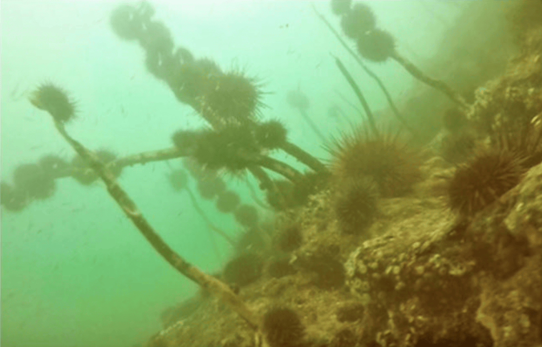
As many of our avid readers already know, the Pacific Coast Feeding Group (PCFG) of gray whales employs a wide range of foraging tactics to feed on a number of different prey items in various benthic substrate types (Torres et al. 2018). One example foraging tactic is when PCFG whales, particularly when they are in the Oregon portion of their feeding range, forage on mysid shrimp in and near kelp beds on rocky reefs. We have countless drone video clips of whales weaving their large bodies through kelp and many photographs of whales coming to the surface to breath completely covered in kelp, looking more like a sea monster than a whale (Figure 1). So, when former intern Dylan Gregory made an astute observation during the 2018 TOPAZ/JASPER field season in Port Orford about a GoPro video the field team collected that showed many urchins voraciously feeding on an unhealthy-looking kelp stalk (Figure 2a), it made us wonder if and how changes to kelp forests may impact gray whales.
Fig 1. Gray whale surfacing in a large kelp patch. Photograph captured under NOAA/NMFS research permit #16111. Source: GEMM Lab.
Kelp forests are widely used as a marine example of trophic cascades. Trophic cascades are trigged by the addition/removal of a top predator to/from a system, which causes changes further down the trophic chain. Sea urchins are common inhabitants of kelp forests and in a balanced, healthy system, urchin populations are regulated by predators as they behave cryptically by hiding in crevices in the reef and individual urchins feed passively on drift kelp that breaks off from larger plants. When we think about who controls urchins in kelp forests, we probably think of sea otters first. However, sea otters have been absent from Oregon waters for over a century (Kone et al. 2021), so who controls urchins here? The answer is the sunflower sea star (Figure 2b). Sunflower sea stars are large predators with a maximum arm span of up to 1 m! Unfortunately, a disease epidemic that started in 2013 known as sea star wasting disease caused 80-100% population decline of sunflower sea stars along the coastline between Mexico and Alaska (Harvell et al. 2019). Shortly thereafter, a record-breaking marine heatwave caused warm, nutrient-poor water conditions to persist in the northeast Pacific Ocean from 2014 to 2016 (Jacox et al. 2018). These co-occurring stressors caused unprecedented and long-lasting decline of a previously robust kelp forest in northern California (Rogers-Bennett & Catton 2019), where sea otters are also absent. Given the biogeographical similarity between southern Oregon and northern California and the observation made by Dylan in 2018, we decided to undertake an analysis of the eight years of data collected during the TOPAZ/JASPER project in Port Orford starting in 2016, to investigate the trends of four trophic levels (purple sea urchins, bull kelp, zooplankton, and gray whales) across space and time. The results of our study were published last week in Scientific Reports and I am excited to be able to share them with you today.
Fig 2a. Sea urchins actively feeding on kelp stalks. Source: GEMM Lab.Fig 2b. Diver holding a sunflower sea star near Port Orford, OR. Source: Scott Groth.
Every day during the TOPAZ/JASPER field season, two teams head out to collect data. One team is responsible for tracking gray whales from shore using a theodolite, while the other team heads out to sea on a tandem research kayak to collect prey data (Figure 3). The kayak team samples prey in multiple ways, including dropping a GoPro camera at each sampling station. When the project was first developed, the original goal of these GoPro videos was to measure the relative abundance of prey. Since the sampling stations occur on or near reefs that are shallow with dense surface kelp, traditional methods to assess prey density, such as using a boat with an echosounder, are not suitable options. Instead, GEMM Lab PI Leigh Torres, together with the first Master’s student on this project Florence Sullivan, developed a method to score still images extracted from the GoPro videos to estimate relative zooplankton abundance. However, after we saw those images of urchins feeding on kelp in 2018, we decided to develop another protocol that allowed us to use these GoPro videos to also characterize sea urchin coverage and kelp condition. Once we had occurrence values for all four species, we were able to dig into the spatiotemporal trends.
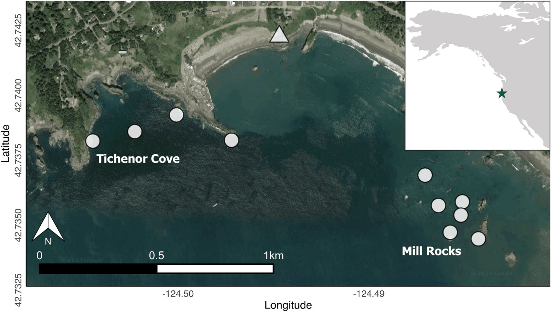
Figure 3. Map of Port Orford, USA study area showing the 10 kayak sampling stations (white circles) within the two study sites (Tichenor Cove and Mill Rocks). The white triangle represents the cliff top location where theodolite tracking of whales was conducted. Figure and caption taken from Hildebrand et al. 2024.
When we examined the trends for each of the four study species across years, we found that purple sea urchin coverage in both of our study sites within Port Orford increased dramatically within our study period (Figure 4). In 2016, the majority of our sampled stations contained no visible urchins. However, by 2020, we detected urchins at every sampling station. For kelp, we saw the reverse trend; in 2016 all sampling stations contained kelp that was healthy or mostly healthy. But by 2019, there were many stations that contained kelp in poor health or where kelp was absent entirely. Zooplankton and gray whales experienced similar temporal trends as the kelp, with their occurrence metrics (abundance and foraging time, respectively) having higher values at the start of our study period and declining steadily during the eight years. While the rise in urchin coverage across our study area occurred concurrently with the decrease in kelp condition, zooplankton abundance, and gray whale foraging, we wanted to explicitly test how these species are related to one another based on prior ecological knowledge.
Figure 4. Temporal trends of purple sea urchin coverage, bull kelp condition, relative zooplankton abundance, and gray whale foraging time by year across the eight-year study period (2016–2023), from the generalized additive models. The colored ribbons represent approximate 95% confidence intervals. Line types represent the two study sites, Mill Rocks (MR; solid) and Tichenor Cove (TC; dashed). All curves are statistically significant (P < 0.05). Figure and caption taken from Hildebrand et al. 2024.
To test whether urchin coverage had an effect on kelp condition, we hypothesized that increased urchin coverage would be correlated with reduced kelp condition based on the decades of research that has established a negative relationship between the two when a trophic cascade occurs in kelp forest systems. Next, we wanted to test whether kelp condition had an effect on zooplankton abundance and hypothesized that increased kelp condition would be correlated with increased zooplankton abundance. We based this hypothesis on several pieces of prior knowledge, particularly as they pertain to mysid shrimp: (1) high productivity within kelp beds provides food for mysids, including kelp zoospores (VanMeter & Edwards 2013), (2) current velocities are one third slower inside kelp beds compared to outside (Jackson & Winant 1983), which might support the retention of mysids within kelp beds since they are not strong swimmers, and (3) the kelp canopy may serve as potential protection for mysids from predators (Coyer 1984). Finally, we wanted to test whether both kelp condition and zooplankton abundance have an effect on gray whales and we hypothesized that increased values for both would be correlated with increased gray whale foraging time. While the reasoning behind our hypothesized correlation between zooplankton prey and gray whales is obvious (whales eat zooplankton), the reasoning behind the kelp-whale connection may not be. We speculated that since kelp habitat may aggregate or retain zooplankton prey, gray whales may use kelp as an environmental cue to find prey patches.
When we tested our hypotheses through generalized additive models, we found that increased urchin coverage was significantly correlated with decreased kelp condition in both study sites, providing evidence that a shift from a kelp forest to an urchin barren may have occurred in the Port Orford area. Additionally, increased kelp condition was correlated with increased zooplankton abundance, supporting our hypothesis that kelp forests are an important habitat and resource for nearshore zooplankton prey. Interestingly, this relationship was bell-shaped in one of our two study sites, suggesting that there are other factors besides healthy bull kelp that influence zooplankton abundance, which likely include upwelling dynamics, habitat structure, and local oceanographic characteristics. For the whale model, we found that increased kelp condition was significantly correlated with increased gray whale foraging time, which may corroborate our hypothesis that gray whales use kelp as an environmental cue to locate prey. Zooplankton abundance was significantly correlated with gray whale foraging time in one of our two sites. Once again, this relationship was bell-shaped, which suggests other factors influence gray whale foraging time, including prey quality (Hildebrand et al. 2022) and density.
Figure 5. Effects derived from trophic path generalized additive models of purple sea urchin coverage on kelp condition (A), kelp condition on relative zooplankton abundance (B), and kelp condition and relative zooplankton abundance on gray whale foraging time (C). The colored ribbons represent approximate 95% confidence intervals. Line types represent the two study sites, Mill Rocks (MR; solid) and Tichenor Cove (TC; dashed). Curves with asterisks indicate statistically significant (P < 0.05) relationships. Figure and caption taken from Hildebrand et al. 2024.
Our results highlight the potential larger impacts of reduced gray whale foraging time as a result of these trophic dynamics may cause at the individual and population level. If an area that was once a reliable source of food (like Port Orford) is no longer favorable, then whales likely search for other areas in which to feed. However, if the areas affected by these dynamics are widespread, then individuals may spend more time searching for, and less time consuming, prey, which could have energetic consequences. While our study took place in a relatively small spatial area, the trophic dynamics we documented in our system may be representative of patterns across the PCFG range, given ecological and topographic similarities in habitat use patterns. In fact, in the years with the lowest kelp, zooplankton, and whale occurrence (2020 and 2021) in Port Orford, the GRANITE field team also noted low whale numbers and minimal surface kelp extent in the central Oregon field site off of Newport. However, ecosystems are resilient. We are hopeful that the dynamics we documented in Port Orford are just short-term changes and that the system will return to its former balanced state with less urchins, more healthy bull kelp, zooplankton, and lots of feeding gray whales.
Did you enjoy this blog? Want to learn more about marine life, research, and conservation? Subscribe to our blog and get a weekly message when we post a new blog. Just add your name and email into the subscribe box below.
References
Coyer, J. A. (1984). The invertebrate assemblage associated with the giant kelp, Macrocystis pyrifera, at Santa Catalina Island, California: a general description with emphasis on amphipods, copepods, mysids, and shrimps. Fishery Bulletin, 82(1), 55-66.
Harvell, C. D., Montecino-Latorre, D., Caldwell, J. M., Burt, J. M., Bosley, K., Keller, A., … & Gaydos, J. K. (2019). Disease epidemic and a marine heat wave are associated with the continental-scale collapse of a pivotal predator (Pycnopodia helianthoides). Science advances, 5(1), eaau7042.
Hildebrand, L., Sullivan, F. A., Orben, R. A., Derville, S., & Torres, L. G. (2022). Trade-offs in prey quantity and quality in gray whale foraging. Marine Ecology Progress Series, 695, 189-201.
Jackson, G. A., & Winant, C. D. (1983). Effect of a kelp forest on coastal currents. Continental Shelf Research, 2(1), 75-80.
Jacox, M. G., Alexander, M. A., Mantua, N. J., Scott, J. D., Hervieux, G., Webb, R. S., & Werner, F. E. (2018). Forcing of multi-year extreme ocean temperatures that impacted California Current living marine resources in 2016. Bull. Amer. Meteor. Soc, 99(1).
Kone, D. V., Tinker, M. T., & Torres, L. G. (2021). Informing sea otter reintroduction through habitat and human interaction assessment. Endangered Species Research, 44, 159-176.
Rogers-Bennett, L., & Catton, C. A. (2019). Marine heat wave and multiple stressors tip bull kelp forest to sea urchin barrens. Scientific reports, 9(1), 15050.
Torres, L. G., Nieukirk, S. L., Lemos, L., & Chandler, T. E. (2018). Drone up! Quantifying whale behavior from a new perspective improves observational capacity. Frontiers in Marine Science, 5, 319.
VanMeter, K., & Edwards, M. S. (2013). The effects of mysid grazing on kelp zoospore survival and settlement. Journal of Phycology, 49(5), 896-901.
By Lindsay Wickman, Postdoc, OSU Department of Fisheries, Wildlife, and Conservation Sciences, Geospatial Ecology of Marine Megafauna Lab
I’ve had the privilege of attending several marine mammal surveys aboard ships at sea, but I had never surveyed for marine mammals from the air. So, when given the opportunity to participate in ongoing aerial surveys off the Oregon Coast with the US Coastguard’s helicopter fleet, I enthusiastically said yes. As Craig Hayslip, a Faculty Research Assistant with the Marine Mammal Institute, prepared me for my first helicopter survey, I was all excitement and no nerves. That is, until he explained the seating arrangement.
“There are two types of helicopters you’ll be flying on, and because of the seating arrangement in the Jayhawk, we fly with the door open when surveying for whales – it’s the only way to get a sufficient view,” Craig casually explained. I stared at the iPad I would use for recording data and imagined it flying through that open door and toward the sea, while I looked on flustered and helpless. Sensing my worry, Craig quickly showed me a set of straps that attached to the iPad, so it could be secured to one of my legs.
In addition to ensuring the iPad stayed in the aircraft, the straps also meant my hands would still be free to handle the camera (to aid in species identification), and a small tool called a geometer (developed by Pi Techology). By lining up the whale sighting in the sight of the geometer, the observer can record the angle between the aircraft and the sighting. Since we also know the height of the helicopter (we fly at a constant altitude of 500 feet), this angle can be used to calculate horizontal distance from the aircraft, allowing an accurate location to be estimated for each sighting.
My first flight was from Warrenton, Oregon, a four-hour drive north from the Hatfield Marine Science Center in Newport. Once at the airport, our first stop was to head to the flight operations office (a.k.a. “Ops”), who set us up with proper clothing and headgear for the flight. As we checked in, rock music played on a speaker while uniformed Coast Guardsmen serviced a helicopter in the hangar. I started to feel like a cool insider, until I clumsily donned the canvas flight suit and tried on several helmets. Suddenly several pounds heavier, all my movements became very awkward.
Lindsay outside the hangar wearing flight gear, in front of the survey’s helicopter. Photo by Craig Hayslip.
After my safety briefing, the entire crew gathered for a pre-flight meeting. We discussed weather conditions, did a wellness check, and discussed the flight’s mission. The conversation also included a brief overview of our scientific aims – why exactly were we looking for whales?
Craig briefly described the research project we were contributing to, titled Overlap Predictions About Large whales (OPAL). The main goal of this project is to better understand the overlap between whales and fisheries, with the aim of reducing entanglement risk. Fishing methods that use fixed, vertical lines in the water column, like the Dungeness crab fishery, can entangle whales as they migrate and feed along Oregon’s coastline. Since reports of whale entanglements have increased on the West Coast in the last 10 years, managing this threat is essential to ensure both the health of whale populations and the stability of Oregon’s crab fishery. Preventing these entanglements requires an understanding of where whales are distributed along the coast, as well as the times of year overlap with fisheries is most likely to occur. The OPAL project isn’t just mapping whale sightings, though. By using models to correlate whale sightings with oceanographic conditions, OPAL is also aiming to predict where whales are likely to occur.
After explaining the mission, the crew had to reach a consensus on both the level of “risk” in the mission and its level of “gain.” For a whale survey flight, risk was deemed low, with medium gain. While I initially felt mild offence that our scientific work was deemed to have just “medium” gain, I quickly reminded myself that when the crew is not flying scientists around, they are literally saving human lives. It was also a reminder that our whale surveys could easily be interrupted if necessary – Craig had mentioned several instances where flights were diverted to assist in rescue or medical emergencies.
With the briefing over, each of us had to consent to the flight plan by saying, “I accept this mission.” I’d heard this phrase from secret agents and soldiers in movies, but never from a marine scientist. I felt out of place saying them at first, but the words undeniably helped me establish a self-assured confidence I would give the survey my 100%.
Finally, it was time to head out of the hangar and to the aircraft. With both a pair of earplugs and my flight helmet on, the whirring of the blades was just a soft hum. I couldn’t hear speech, so we all relied on hand signals to communicate until our headsets were connected to the aircraft. The crew helped make sure I correctly put on my seatbelt harness, which had not just one, but five buckles. While I still felt some mild concern for the iPad strapped to my leg, at least I knew I wouldn’t fall out.
Preparing for takeoff. Photo by Craig Hayslip.Lindsay holds up the geometer during the flight. Photo by Craig Hayslip.
Craig helped ensure I had all the equipment set up properly: the iPad’s survey program, the GPS tracking, and the computer recording the geometer’s measurements. Soon after, the helicopter slowly rose, hovering above the runway, before turning and heading towards the coast at speed. My stomach dropped slightly, my ears popped, and cold air rushed through the open door. I looked out at the Columbia River as it stretched toward the coastline and out to sea, and I couldn’t stop smiling.
A rainbow mid-air. Photo by Craig Hayslip.
As we approached the ocean, my attention shifted back to the mission, and I started scanning the surface for whale blows. With the large helmet on, I noticed the camera and geometer were much more difficult to use, so I also made “practice sightings” of passing boats and buoys. It didn’t take long before my first real whale sighting though – two gray whales (Eschrichtius robustus). Over the next two hours, I saw four more gray whales, and six more whales I was unable to identify due to distance. With each sighting, I had to act fast to make each geometer recording. The helicopter travels at a speed of 90 knots and whales can disappear soon after surfacing.
Two hours of flying with the door open meant my nose was running and my typing skills were worsening due to cold fingers. As exciting as it was to spot whales from the air, I was a little relieved when we arrived back at the airport and I could warm back up. Luckily, my nightmare of losing an iPad from the helicopter did not come true, and I was returning home with another survey to add to over 200 (and counting!) helicopter surveys completed for the OPAL project. Four different flights covering different parts of the Oregon coast are completed each month, so I know I have more flights to look forward to. After a successful first mission, I feel ready to take on my next flight.
The four flight routes completed monthly for the OPAL project. Helicopter flights are enabled through a partnership with the US Coastguard.
If you’d like to learn more about the OPAL research project, check out these past blog posts:
Recent publications presenting findings from the first two years of OPAL include:
Derville, S., Barlow, D. R., Hayslip, C., & Torres, L. G. (2022). Seasonal, Annual, and Decadal Distribution of Three Rorqual Whale Species Relative to Dynamic Ocean Conditions Off Oregon, USA. Frontiers in Marine Science, 9. https://doi.org/10.3389/fmars.2022.868566
Derville, S., Buell, T. v., Corbett, K. C., Hayslip, C., & Torres, L. G. (2023). Exposure of whales to entanglement risk in Dungeness crab fishing gear in Oregon, USA, reveals distinctive spatio-temporal and climatic patterns. Biological Conservation, 281. https://doi.org/10.1016/j.biocon.2023.10998
Did you enjoy this blog? Want to learn more about marine life, research, and conservation? Subscribe to our blog and get a weekly message when we post a new blog. Just add your name and email into the subscribe box below.
Imagine you are 50 nautical miles from shore, perched on the observation platform of a research vessel. The ocean is blue, calm, and seems—for all intents and purposes—empty. No birds fly overhead, nothing disturbs the rolling swells except the occasional whitecap from a light breeze. The view through your binoculars is excellent, and in the distance, you spot a disturbance at the surface of the water. As the ship gets closer, you see splashing, and a flurry of activity emerges as a large group of dolphins leap and dive, likely chasing a school of fish. They swim along with the ship, riding the bow-wave in a brief break from their activity. Birds circle in the air above them and float on the water around them. Together with your team of observers, you rush to record the species, the number of animals, their distance to the ship, and their behavior. The research vessel carries along its pre-determined trackline, and the feeding frenzy of birds and dolphins fades off behind you as quickly as it came. You return to scanning the blue water.
Craig Hayslip and Dawn Barlow scan for marine mammals from the crow’s nest (elevated observation platform) of the R/V Pacific Storm.
The marine environment is highly dynamic, and resources in the ocean are notoriously patchy. One of our main objectives in marine ecology is to understand what drives these ephemeral hotspots of species diversity and biological activity. This objective is particularly important now as the oceans warm and shift. In the context of rapid global climate change, there is a push to establish alternatives to fossil fuels that can support society’s energy needs while minimizing the carbon emissions that are a root cause of climate change. One emergent option is offshore wind, which has become a hot topic on the West Coast of the United States in recent years. The technology has the potential to supply a clean energy source, but the infrastructure could have environmental and societal impacts of its own, depending on where it is placed, how it is implemented, and when it is operational.
Northern right whale dolphins leap into the air. Photo by Craig Hayslip.
Any development in the marine environment, including alternative energy such as offshore wind, should be undertaken using the best available scientific knowledge of the ecosystem where it will be implemented. The Marine Mammal Institute’s collaborative project, Marine Offshore Species Assessments to Inform Clean energy (MOSAIC), was designed for just this reason. As the name “MOSAIC” implies, it is all about using different tools to compile different datasets to establish crucial baseline information on where marine mammals and seabirds are distributed in Oregon and Northern California, a region of interest for wind energy development.
A MOSAIC of species
The waters of Oregon and Northern California are rich with life. Numerous cetaceans are found here, from the largest species to ever live, the blue whale, to one of the smallest cetaceans, the harbor porpoise, with many species filling in the size range in between: fin whales, humpback whales, sperm whales, killer whales, Risso’s dolphins, Pacific white-sided dolphins, northern right whale dolphins, and Dall’s porpoises, to name a few. Seabirds likewise rely on these productive waters, from the large, graceful albatrosses that feature in maritime legends, to charismatic tufted puffins, to the little Leach’s storm petrels that could fit in the palm of your hand yet cover vast distances at sea. From our data collection efforts so far, we have already documented 16 cetacean species and 64 seabird species.
A Laysan albatross glides over the water’s surface. Photo by Will Kennerley.
A MOSAIC of data and tools
Schematic of the different components of the MOSAIC project. Graphic created by Solene Derville.
Through the four-year MOSAIC project, we are undertaking two years of visual surveys and passive acoustic monitoring from Cape Mendocino to the mouth of the Columbia River on the border of Oregon and Washington and seaward to the continental slope. Six comprehensive surveys for cetaceans and seabirds are being conducted aboard the R/V Pacific Storm following a carefully chosen trackline to cover a variety of habitats, including areas of interest to wind energy developers.
These dedicated surveys are complemented by additional surveys conducted aboard NOAA research vessels during collaborative expeditions in the Northern California Current, and ongoing aerial surveys in partnership with the United States Coast Guard through the GEMM Lab’s OPAL project. Three bottom-mounted hydrophones were deployed in August 2022, and are recording cetacean vocalizations and the ambient soundscape, and these recordings will be complemented by acoustic data that is being collected continuously by the Oceans Observing Initiative. In addition to these methods to collect broad-scale species distribution information, concurrent efforts are being conducted via small boats to collect individual identification photographs of baleen whales and tissue biopsy samples for genetic analysis. Building on the legacy of satellite tracking here at the Marine Mammal Institute, the MOSAIC project is breathing new life into tag data from large whales to assess movement patterns over many years and determine the amount of time spent within our study area.
A curious fin whale approaches the R/V Pacific Storm during one of the visual surveys. Photo by Craig Hayslip.
Survey tracklines extending between the Columbia River and Cape Mendocino, designed for the MOSAIC visual surveys aboard the R/V Pacific Storm.
The resulting species occurrence data from visual surveys and acoustic monitoring will be integrated to develop Species Distribution Models for the many different species in our study region. Identification photographs of individual baleen whales, DNA profiles from whale biopsy samples, and data from satellite-tagged whales will provide detailed insight into whale population structure, behavior, and site fidelity (i.e., how long they typically stay in a given area), which will add important context to the distribution data we collect through the visual surveys and acoustic monitoring. The models will be implemented to produce maps of predicted species occurrence patterns, describing when and where we expect different cetaceans and seabirds to be under different environmental conditions.
With five visual surveys down, the MOSAIC team is gearing up for one final survey this month. The hydrophones will be retrieved this summer. Then, with data in-hand, the team will dive deep into analysis.
A MOSAIC of collaborators
The MOSAIC-4 team waves from the crow’s nest (observation platform) of the R/V Pacific Storm. Photo by Craig Hayslip.
The collaborative MOSAIC team brings together a diverse set of tools. The depth of expertise here at the Marine Mammal Institute spans a broad range of disciplines, well-positioned to provide robust scientific knowledge needed to inform alternative energy development in Oregon and Northern California waters.
I have had the pleasure of participating in three of the six surveys aboard the R/V Pacific Storm, including leading one as Chief Scientist, and have collected visual survey data aboard NOAA Ship Bell M. Shimada and from United States Coast Guard helicopters over the years that will be incorporated in the MOSAIC of datasets for the project. This ecosystem is one that I feel deeply connected to from time spent in the field. Now, I am thrilled to dive into the analysis, and will lead the modeling of the visual survey data and the integration of the different components to produce species distribution maps for cetaceans and seabirds our study region.
This project is funded by the United States Department of Energy. The Principal Investigator is the Institute’s Director Dr. Lisa Ballance, and Co-Principal Investigators include Scott Baker, Barbara Lagerquist, Rachael Orben, Daniel Palacios, Kate Stafford, and Leigh Torres of the Marine Mammal Institute; John Calambokidis of the Cascadia Research Collective; and Elizabeth Becker of ManTech International Corp. For more information, please visit the project website, and stay tuned for updates as we enter the analysis phase.
Did you enjoy this blog? Want to learn more about marine life, research, and conservation? Subscribe to our blog and get a weekly alert when we make a new post! Just add your name into the subscribe box below!