Dawson Mohney, TOPAZ/JASPER HS Intern, Pacific High School Graduate
My name is Dawson Mohney, I am a high school intern for the 2025 TOPAZ/JASPER team this field season. I first heard about the TOPAZ/JASPER internship from my friend Jonah Lewis, a previous intern from the 2023 field season. Coincidentally, Jonah and I both graduated this year from Pacific High School here on the coast—small world. I have called Port Orford my home for most of my life, and in recent years I discovered that a gray whale research project has been happening in my own backyard. Growing up less than a mile from the Oregon Coast, I’ve spent a lot of time looking out into the water. I always liked how, no matter what happened in my life, the ocean was always there. This interest is what encouraged me to apply for the internship with the hope of discovering more about the ocean, a substantial part of my home and family.
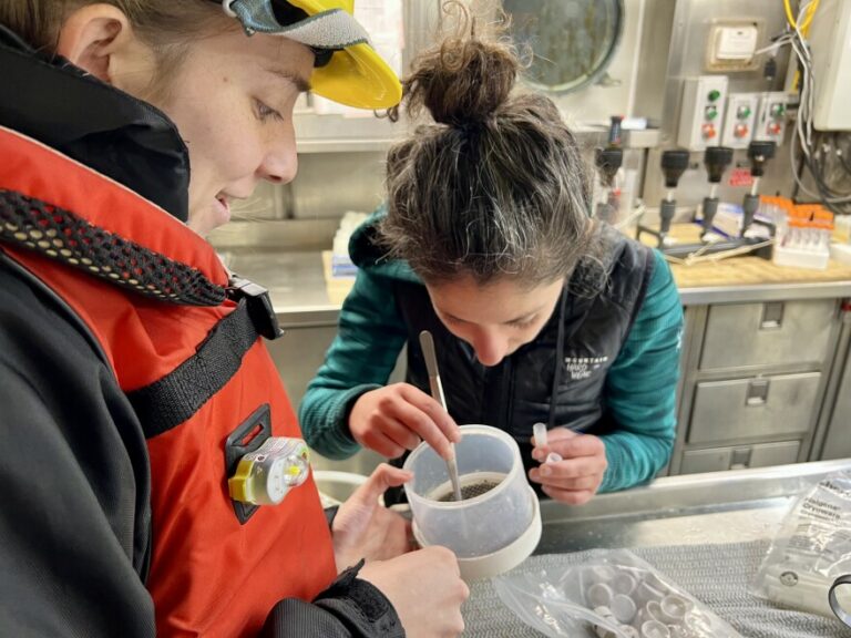
Fig 1: Picture fellow intern Maddie took of me (Dawson) during our trip to Natural Bridges.
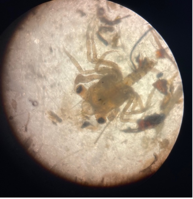
A critical part of this project is understanding not only the magnificent gray whales but also the much less apparent zooplankton–after all, the whales need to eat a lot of zooplankton! Many different species of zooplankton—“zoop” for short—call the Oregon coast home. Each day, as we kayak to our 12 sample stations within the gray whale feeding grounds of Mill Rocks and Tichenor’s Cove, I find myself wondering which species of zoop I’ll get to identify later under the microscope.
Throughout the duration of this internship, our team has met to discuss a few research papers published by GEMM Lab members, including research produced from the TOPAZ/JASPER projects. Recently, I read, “Do Gray Whales Count Calories? Comparing Energetic Values of Gray Whale Prey Across Two Different Feeding Grounds in the Eastern North Pacific,” by Hildebrand et al. who describe the caloric content of different zooplankton species. Before reading this paper, I didn’t realize whale prey could vary in nutritional value – much like food for humans. This paper made it clear that each of the different species of zooplankton is just as important as the last, but consuming more of the higher caloric species such as the Neomysis rayii or the Dungeness crab larvae would certainly be a welcome meal. Seeing these “healthy” meals in the area makes me hopeful for the whales.
Fig 2: Image of a crab larvae in their megalopae stage.
From reading previous blog posts, the foraging habits of the whales this season appear to be unusual. In prior TOPAZ/JASPER field seasons, gray whales have often been tracked foraging near or around our Mill Rocks and Tichenor Cove study sites. This season, we haven’t tracked a single whale in Mill Rocks and only two in Tichenor Cove. Could there just not be enough good zoop?
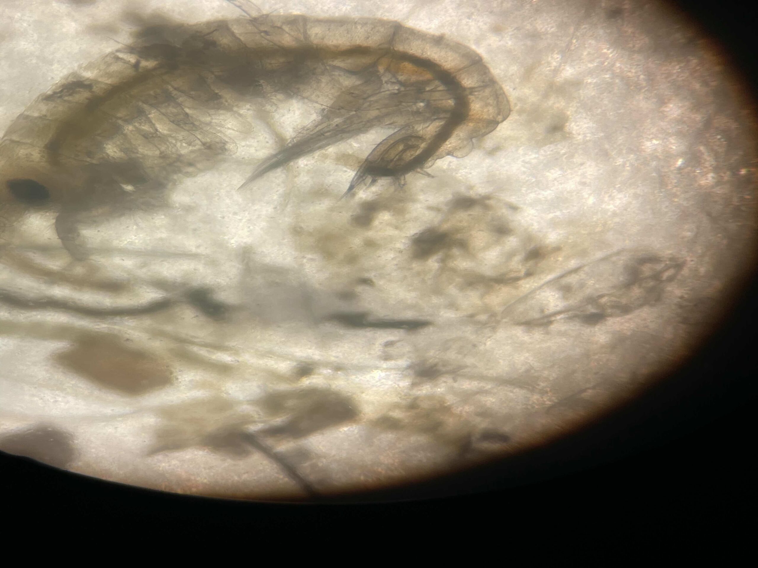
Along with this lack of whales, there does seem to be a lack of these “high calorie zoop species”. Our team has most frequently collected samples primarily comprising of Atylus tridens, a lower calorie prey type. In fact, during one of our earlier kayak training days this field season we collected 2,019 individual A. tridens. However, since this day we have collected sparse amounts of zooplankton in our samples, ranging from zero to 121 in a given sample. Our total zoop count thus far is 2,524 zooplankton, a third of the total zooplankton collected last field season.
Fig 3: Image of an Atylus tridens under a microscope.
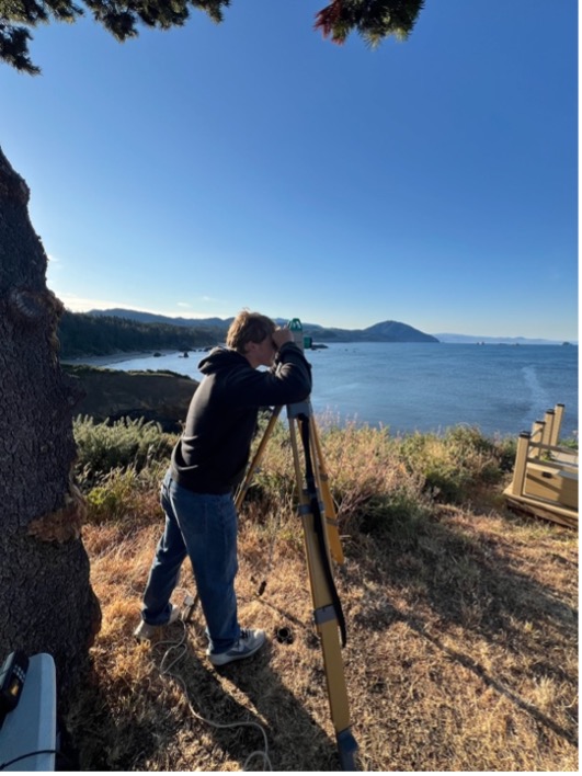
As for whale presence, we have been observing many whales blows near Hell’s Gate as mentioned in last week’s blog written by fellow intern Miranda Fowles. From our cliff site, it has been difficult to know whether these are gray whales or a different kind of whale, leading us to venture out to the Heads to get a better look. The persistence of whales in this area is certainly unusual, and perhaps it can be explained by a larger amount of higher calorie zooplankton species in the Hell’s Gate area.
Fig 4: Dawson tracking blows by Hell’s Gate with the theodolite.
Being part of the TOPAZ/JASPER project, I have become exposed to what the true meaning is behind “fieldwork,” including learning how to be flexible and adapt to new challenges every day. What I have most enjoyed is the team’s ability to overcome any new hurdle together as a unit. My dad often says, “You learn something new every day,” and this internship couldn’t embody this quote more. In just these 5 weeks, it almost feels like my head is now a couple sizes bigger.
Before this experience, I never thought much about how one might track a whale or how different microscopic species could have such a profound impact on a whale’s decision to forage. Now I feel I understand just how important these less than obvious factors are and the effort which goes behind understanding these relationships. I can only hope future opportunities teach me as much as joining the TOPAZ/JASPER legacy has—it’s an experience that, even just a few days into the 2025 field season, I knew would be hard to match.
Fig 4: Dawson (navigator) and Miranda (sampler) during kayak training on their way to Mill Rocks.
Hildebrand, L., Bernard, K. S., & Torres, L. G. (2021). Do Gray Whales Count Calories? Comparing Energetic Values of Gray Whale Prey Across Two Different Feeding Grounds in the Eastern North Pacific. Frontiers in Marine Science, 8, 683634. https://doi.org/10.3389/fmars.2021.683634
By Rachel Kaplan, PhD candidate, Oregon State University College of Earth, Ocean, and Atmospheric Sciences and Department of Fisheries, Wildlife, and Conservation Sciences, Geospatial Ecology of Marine Megafauna Lab
At the beginning of a graduate program, it’s common for people to tell you how quickly the time will pass, but hard to imagine that will really be the case. Suddenly, I’ve been working on my PhD for almost five years, and I’ll defend in just over two weeks. As I look back, I am amazed by how much I have learned and grown during this time, and how all the different parts of my graduate school experience have woven together. I began my program in 2020 with an intense “bootcamp” of oceanographic coursework, and am ending in 2025 with new analytical skills, a few publications, and a ton of new thoughts about whales and the zooplankton krill, the subjects of my research. My PhD work encapsulates all those different elements in an exploration of ecological relationships between baleen whale predators and their krill prey – which I now see as an expression of oceanographic and atmospheric processes.
Figure 1. One of my favorite sightings during my PhD fieldwork was a group of seven fin whales in Antarctica, on Christmas 2024. Photo: Rachel Kaplan
Oceanographic processes drive prey quantity and quality across time and space, shaping the preyscape encountered by predators on their foraging grounds and driving habitat use (Fleming et al., 2016; Ryan et al., 2022). Aspects of prey including distribution, energy density, and biomass therefore represent mechanistic links between ocean and atmospheric conditions (e.g., El Niño Southern Oscillation cycles, circulation patterns, and upwelling processes) and diverse aspects of marine predator ecology, including spatiotemporal distributions, foraging behaviors, reproductive success, population size, and health. Both predator and prey species are impacted by environmental variability and climate change (e.g., Hauser et al., 2017; Atkinson et al., 2019; Perryman et al., 2021), and events like marine heatwaves and harmful algal blooms can force ecosystem changes on short, seasonal time scales (e.g. McCabe et al., 2016; Fisher et al., 2020). However, many marine species have some degree of plasticity that allows them to still accomplish life history events in the face of ecosystem variability (e.g., Lawrence, 1976; Oestreich, 2022), which may provide the capacity to adapt to climate change processes.
Observing and describing predator-prey relationships is complex due to the scale-dependent nature of these relationships (Levin, 1992). Each chapter of my dissertation considered krill, a globally-important prey type, from the perspective of baleen whales, which are krill predators. Chapter 2 used a comparative analysis to identify the optimal spatial scale at which to observe baleen whale-krill relationships on the Northern California Current (NCC) foraging grounds. We found correlations at a 5 km scale to be strongest, which can provide a useful starting point for further studies in the NCC and other systems. Chapter 3 used this spatial scale to compare several aspects of krill prey quality and quantity as predictors of humpback whale (Megaptera novaeangliae) distributions in the NCC. The best performing metric was a species, season, and spatially informed krill swarm biomass variable – yet the comparable performance of a simple acoustic abundance metric indicated that it can act as a reliable proxy for biomass. This finding may be advantageous for future research, as measuring the acoustic proxy is less computationally intensive and relies on fewer datastreams. Interestingly, one of this study’s best-performing models was based on only the proportion of Thysanoessa spinifera in krill swarms, which is also a highly accessible variable due to effective krill species distribution modeling in the NCC (Derville et al., 2024). Integrating the acoustic abundance proxy and krill species distribution predictions, two relatively simple metrics, could support predictions of humpback whale distributions in the NCC and inform whale-prey research in other ecosystems.
Figure 2. Collecting samples of individual krill gave us the opportunity to learn about their quality as prey for whales in the Northern California Current. Photo: Courtney Flatt
Studies relating predator foraging to prey characteristics often rely on metrics such as prey biomass or energy density (Schrimpf et al., 2012; Savoca et al., 2021; Cade et al., 2022), but the tendency of krill to form aggregations introduces dimensionality to krill prey quality. Chapter 4 showed that elements of krill swarm structure (particularly depth, proportion of T. spinifera, and metrics describing how krill occupy space within swarms) may be mechanistic drivers of variable blue, fin and humpback whale distribution patterns on the NCC foraging grounds. These findings suggest that krill swarm characteristics may be important links between baleen whales and the foraging environment. Swarm characteristics may be considered a component of krill prey quality for baleen whales, and future research could illuminate direct causal relationships between oceanographic conditions, krill swarming responses, and niche expression in baleen whale predators.
The relationships between baleen whale distributions and krill quantity and quality explored in the first chapters of my dissertation may also shed light on other aspects of baleen whale ecology. The final chapter considers overwintering trends in global baleen whale populations, and examines the wintertime Western Antarctic Peninsula (WAP) as a case study. Extended humpback whale presence on the WAP feeding grounds may be driven by the profitable feeding areas and elevated energy content of krill during the winter months, and may reflect the high energetic needs of certain demographic subgroups (e.g. lactating females, juveniles). Wintertime humpback whale presence may also reflect adaptation to multifaceted competitive pressure on krill resources that are declining due to climate change (Atkinson et al., 2019), including consumption by growing baleen whale populations (Johnston et al., 2011) and a fishery whose catch limits may be impacting krill predators (Watters et al., 2020; Savoca et al., 2024). This work demonstrates how investigating prey quality during the winter months can contextualize baleen whale overwintering on the foraging grounds. It also provides a meaningful violation of the canonical baleen whale migration paradigm central to marine mammal science, which may lessen the efficacy of whale monitoring programs and management policies.
Figure 3. We were surprised to see humpback whales like this one in Antarctica during the winter months — which raised a number of questions about overwintering of baleen whales on foraging grounds around the world. Photo: Giulia Wood
Management efforts that aim to mitigate risk to whales often hinge on predictive modeling of whale distributions. Species distribution models (SDMs) can provide managers with spatially and temporally explicit predictions of protected species occurrences (Wikgren et al., 2014; Santora et al., 2020), but species distributions in rapidly changing ecosystems are difficult to predict (Muhling et al., 2020). Findings from this dissertation may inform modeling efforts by suggesting meaningful predictor variables for SDMs, such as krill species on the NCC foraging grounds and swarm energy density at the WAP. This work also speaks to meaningful spatial scales for analyzing predator-prey relationships (i.e., 5 km), and relevant elements of temporal variability (e.g., seasonal cycles of krill energy density).
Just as marine predator-prey relationships are shaped by ocean processes, they likewise have consequences for those processes. For example, krill and other zooplankton are capable of generating large-scale mixing that can overcome stratification of water masses and alter water column structure (Noss and Lorke, 2014). Baleen whales influence global carbon cycles due to the huge amount of prey they consume (Savoca et al., 2021; Pearson et al., 2023) and transport important nutrients along the “great whale conveyer belt” during their vast migrations (Roman et al., 2025). Baleen whales seek krill as an essential prey resource on foraging grounds around the globe, and the impact of this trophic interaction scales up, with implications for ecosystem functioning and management. Continued research into the spatiotemporally dynamic relationships between krill and baleen whales improves our understanding of ocean functioning, and can improve our capacity to live as part of this system.
References
Atkinson, A., Hill, S. L., Pakhomov, E. A., Siegel, V., Reiss, C. S., Loeb, V. J., Steinberg, D. K., et al. 2019. Krill (Euphausia superba) distribution contracts southward during rapid regional warming. Nature Climate Change, 9: 142–147.
Cade, D. E., Kahane-Rapport, S. R., Wallis, B., Goldbogen, J. A., and Friedlaender, A. S. 2022. Evidence for Size-Selective Predation by Antarctic Humpback Whales. Frontiers in Marine Science, 9: 747788.
Derville, S., Fisher, J. L., Kaplan, R. L., Bernard, K. S., Phillips, E. M., and Torres, L. G. 2024. A predictive krill distribution model for Euphausia pacifica and Thysanoessa spinifera using scaled acoustic backscatter in the Northern California Current. Progress in Oceanography: 103388.
Fisher, J. L., Menkel, J., Copeman, L., Shaw, C. T., Feinberg, L. R., and Peterson, W. T. 2020. Comparison of condition metrics and lipid content between Euphausia pacifica and Thysanoessa spinifera in the northern California Current, USA. Progress in Oceanography, 188.
Fleming, A. H., Clark, C. T., Calambokidis, J., and Barlow, J. 2016. Humpback whale diets respond to variance in ocean climate and ecosystem conditions in the California Current. Glob Chang Biol, 22: 1214–24.
Hauser, D. D. W., Laidre, K. L., Stafford, K. M., Stern, H. L., Suydam, R. S., and Richard, P. R. 2017. Decadal shifts in autumn migration timing by Pacific Arctic beluga whales are related to delayed annual sea ice formation. Global Change Biology, 23: 2206–2217.
Johnston, S. J., Zerbini, A. N., and Butterworth, D. S. 2011. A Bayesian approach to assess the status of Southern Hemipshere humpback whales (Megaptera novaeangliae) with an application to Breeding Stock G. J. Cetacean Res. Manage.: 309–317. International Whaling Commission.
Lawrence, J. M. 1976. Patterns of Lipid Storage in Post-Metamorphic Marine Invertebrates. American Zoologist, 16: 747–762. Oxford University Press (OUP).
Levin, S. A. 1992. The Problem of Pattern and Scale in Ecology: The Robert H. MacArthur Award Lecture. Ecology, 73: 1943–1967.
McCabe, R. M., Hickey, B. M., Kudela, R. M., Lefebvre, K. A., Adams, N. G., Bill, B. D., Gulland, F. M., et al. 2016. An unprecedented coastwide toxic algal bloom linked to anomalous ocean conditions. Geophys Res Lett, 43: 10366–10376.
Muhling, B. A., Brodie, S., Smith, J. A., Tommasi, D., Gaitan, C. F., Hazen, E. L., Jacox, M. G., et al. 2020. Predictability of Species Distributions Deteriorates Under Novel Environmental Conditions in the California Current System. Frontiers in Marine Science, 7.
Noss, C., and Lorke, A. 2014. Direct observation of biomixing by vertically migrating zooplankton. Limnology and Oceanography, 59: 724–732. Wiley.
Oestreich, W. 2022. Acoustic signature reveals blue whales tune life‐history transitions to oceanographic conditions. Functional Ecology. https://besjournals.onlinelibrary.wiley.com/doi/10.1111/1365-2435.14013 (Accessed 20 September 2024).
Pearson, H. C., Savoca, M. S., Costa, D. P., Lomas, M. W., Molina, R., Pershing, A. J., Smith, C. R., et al. 2023. Whales in the carbon cycle: can recovery remove carbon dioxide? Trends in Ecology & Evolution, 38: 238–249.
Perryman, W. L., Joyce, T., Weller, D. W., and Durban, J. W. 2021. Environmental factors influencing eastern North Pacific gray whale calf production 1994–2016. Marine Mammal Science, 37: 448–462. Wiley.
Roman, J., Abraham, A. J., Kiszka, J. J., Costa, D. P., Doughty, C. E., Friedlaender, A., Hückstädt, L. A., et al. 2025. Migrating baleen whales transport high-latitude nutrients to tropical and subtropical ecosystems. Nature Communications, 16: 2125. Nature Publishing Group.
Ryan, J. P., Benoit-Bird, K. J., Oestreich, W. K., Leary, P., Smith, K. B., Waluk, C. M., Cade, D. E., et al. 2022. Oceanic giants dance to atmospheric rhythms: Ephemeral wind-driven resource tracking by blue whales. Ecology Letters, 25: 2435–2447.
Santora, J. A., Mantua, N. J., Schroeder, I. D., Field, J. C., Hazen, E. L., Bograd, S. J., Sydeman, W. J., et al. 2020. Habitat compression and ecosystem shifts as potential links between marine heatwave and record whale entanglements. Nat Commun, 11: 536.
Savoca, M. S., Czapanskiy, M. F., Kahane-Rapport, S. R., Gough, W. T., Fahlbusch, J. A., Bierlich, K. C., Segre, P. S., et al. 2021. Baleen whale prey consumption based on high-resolution foraging measurements. Nature, 599: 85–90.
Savoca, M. S., Kumar, M., Sylvester, Z., Czapanskiy, M. F., Meyer, B., Goldbogen, J. A., and Brooks, C. M. 2024. Whale recovery and the emerging human-wildlife conflict over Antarctic krill. Nature Communications, 15: 7708. Nature Publishing Group.
Schrimpf, M., Parrish, J., and Pearson, S. 2012. Trade-offs in prey quality and quantity revealed through the behavioral compensation of breeding seabirds. Marine Ecology Progress Series, 460: 247–259.
Watters, G. M., Hinke, J. T., and Reiss, C. S. 2020. Long-term observations from Antarctica demonstrate that mismatched scales of fisheries management and predator-prey interaction lead to erroneous conclusions about precaution. Scientific Reports, 10: 2314.
Wikgren, B., Kite-Powell, H., and Kraus, S. 2014. Modeling the distribution of the North Atlantic right whale Eubalaena glacialis off coastal Maine by areal co-kriging. Endangered Species Research, 24: 21–31.
Dr. Enrico Pirotta (CREEM, University of St Andrews) and Dr. Leigh Torres (GEMM Lab, MMI, OSU)
The health of animals affects their ability to survive and reproduce, which, in turn, drives the dynamics of populations, including whether their abundance trends up or down. Thus, understanding the links between health and reproduction can help us evaluate the impact of human activities and climate change on wildlife, and effectively guide our management and conservation efforts. In long-lived species, such as whales, once a decline in population abundance is detected, it can be too late to reverse the trend, so early warning signals are needed to indicate how these populations are faring.
We worked on this complex issue in a study that was recently published in the Journal of Animal Ecology. In this paper, we developed a new statistical approach to link three key components of the health of a Pacific Coast Feeding Group (PCFG) gray whale (namely, its body size, body condition, and stress levels) to a female’s ability to give birth to a calf. We were able to inform these metrics of whale health using an eight-year dataset derived from the GRANITE project of aerial images from drones for measurements of body size and condition, and fecal samples for glucocorticoid hormone analysis as an indicator of stress. We combined these data with observations of females with or without calves throughout the PCFG range over our study period.
We found that for a female to successfully have a calf, she needs to be both large and fat, as these factors indicate if the female has enough energy stored to support reproduction that year (Fig. 1). Remarkably, we also found indication that females with particularly high stress hormone levels may not get pregnant in the first place, which is the first demonstration of a link between stress physiology and vital rates in a baleen whale, to our knowledge.
Figure 1. Taken from Pirotta et al. (2025), Fig. 5. Combined relationship of PCFG gray whale length and nutritional state (combination of body size and condition) in the previous year with calving probability, colored by whether the model estimated an individual to have calved or not at a given reproductive opportunity.
Our study’s findings are concerning given our previous research indicating that gray whales in this PCFG sub-group have been growing to shorter lengths over the last couple of decades (Pirotta et al. 2023), are thinner than animals in the broader Eastern North Pacific gray whale population (Torres et al, 2022), and show an increase in stress-related hormones when exposed to human activities (Lemos et al, 2022; Pirotta et al. 2023). Furthermore, in our recent study we also documented that there are fewer young individuals than expected for a growing or stable population (Fig. 2), which can be an indicator of a population in decline since there may not be many individuals entering the reproductive adult age groups. Altogether, our results act as early warning signals that the PCFG may be facing a possible population decline currently or in the near future.
Figure 2. Taken from Pirotta et al. (2025), Fig. 1. Age structure diagram for 139 PCFG gray whales in our dataset. Each bar represents the number of individuals of a given age in 2023, with the color indicating the proportion of individuals of that age for which age is known (vs. estimated from a minimum estimate following Pirotta, Bierlich, et al., 2024). The red line reports a smooth kernel density estimate of the distribution.
These findings are sobering news for Oregon residents and tourists who enjoy watching these whales along our coast every summer and fall. We have gotten to know many of these whales so well – like Scarlett, Equal, Clouds, Lunita, and Pacman, who you can meet on our IndividuWhale website – that we wonder how they will adapt and survive as their once reliable habitat and prey-base changes. We hope our work sparks collective and multifaceted efforts to reduce impacts on these unique PCFG whales, and that we can continue the GRANITE project for many more years to come to monitor these whales and learn from their response to change.
This work exemplifies the incredible value of long-term studies, interdisciplinary methods, and effective collaboration. Through many years of research on this gray whale group, we have collected detailed data on diverse aspects of their behavior, ecology and life history that are critical to understanding their response to disturbance and environmental change, which are both escalating in the study region. We are incredibly grateful to the following members of the PCFG Consortium for contributing sightings and calf observation data that supported this study: Jeff Jacobsen, Carrie Newell, NOAA Fisheries (Peter Mahoney and Jeff Harris), Cascadia Research Collective (Alie Perez), Department of Fisheries and Oceans, Canada (Thomas Doniol-Valcroze and Erin Foster), Mark Sawyer and Ashley Hoyland, Wendy Szaniszlo, Brian Gisborne, Era Horton.
Did you enjoy this blog? Want to learn more about marine life, research, and conservation? Subscribe to our blog and get a weekly alert when we make a new post! Just add your name into the subscribe box below!
References:
Lemos, Leila S., Joseph H. Haxel, Amy Olsen, Jonathan D. Burnett, Angela Smith, Todd E. Chandler, Sharon L. Nieukirk, Shawn E. Larson, Kathleen E. Hunt, and Leigh G. Torres. “Effects of Vessel Traffic and Ocean Noise on Gray Whale Stress Hormones.” Scientific Reports 12, no. 1 (2022): 18580. https://dx.doi.org/10.1038/s41598-022-14510-5.
Pirotta, Enrico, Alejandro Fernandez Ajó, K. C. Bierlich, Clara N Bird, C Loren Buck, Samara M Haver, Joseph H Haxel, Lisa Hildebrand, Kathleen E Hunt, Leila S Lemos, Leslie New, and Leigh G Torres. “Assessing Variation in Faecal Glucocorticoid Concentrations in Gray Whales Exposed to Anthropogenic Stressors.” Conservation Physiology 11, no. 1 (2023). https://dx.doi.org/10.1093/conphys/coad082.
Torres, Leigh G., Clara N. Bird, Fabian Rodríguez-González, Fredrik Christiansen, Lars Bejder, Leila Lemos, Jorge Urban R, et al. “Range-Wide Comparison of Gray Whale Body Condition Reveals Contrasting Sub-Population Health Characteristics and Vulnerability to Environmental Change.” Frontiers in Marine Science 9 (2022). https://doi.org/10.3389/fmars.2022.867258. https://www.frontiersin.org/article/10.3389/fmars.2022.867258
Baleen whales must navigate a seemingly featureless world to locate the resources they need to survive. The task of finding prey to feed on in the vast seascapes relies on the use of several sensory modalities that operate at different scales (Torres 2017; Figure 1). For example, baleen whale vision is believed to be rather limited, with the ability to see objects about 10-100 meters away. Yet, baleen whale somatosensory perception of oceanographic stimuli is thought to be on the order of 100-1000s kilometers. This diversity in sensory ability has led scientists to believe that whales, in fact all animals, perceive cues and make decisions at several scales. As ecologists, we endeavor to understand why and when animals are found (or not found) in certain locations as this knowledge allows us to better manage and conserve animal populations. With this information we can aim to minimize potential anthropogenic disturbance and protect important resource areas, such as foraging or nursing grounds. In order to accomplish this goal, we ourselves must conduct studies and test hypotheses at several scales (Levin 1992; Hobbs 2003). As someone who tackles spatial foraging ecology questions, I am particularly interested in understanding whale behavior and movement in the context of feeding. Since accurately measuring predator and prey distribution at the same scales can be challenging, we often resort to environmental variables to serve as proxies for prey, whereby we look for correlations between environmental variables and whales to understand and predict the distribution of our population.
Figure 1. Schematic of hypothetical interchange of sensory modalities used by baleen whales to locate prey at variable scales. X-axis represents log distance to prey from micro (left) to macro (right). Y-axis represents the relative use of each sensory modality between 0 (no contribution) to 10 (highest contribution). Each line and color represent a different sensory modality. Figure taken and caption adapted from Torres 2017.
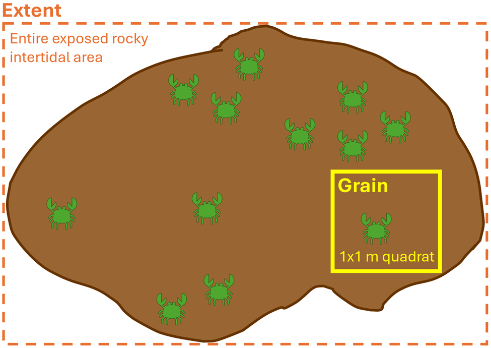
What do I mean when I use the word ‘scale’? The term scale is typically explained by two components: grain and extent (Wiens 1989). The grain is the finest resolution measured; in other words, how detailed we are measuring. The extent is the overall coverage of what we are measuring. These components can be applied to both spatial scale and temporal scale. For example, spatially, if we were using a 1×1 meter sampling quadrat to count the number of crabs on a rocky shore, then our grain would be the 1 m2 quadrat and the extent would be the entire exposed rocky intertidal area that we are surveying (Figure 2). Temporally, if we placed a temperature logger at the mouth of Yaquina Bay that took a temperature recording every minute for two years, then our grain would be one minute and the extent would be two years. So, when designing a study, it is imperative for us to decide on the spatiotemporal scales of the ecological questions we are asking and the hypotheses we are testing, as it will inform what data we need to collect. When making this decision, it is important to think about the scale at which the ecological process happens, as opposed to the scale at which we can observe the process (Levin 1992). In other words, we need to think from the perspective of our study species, as opposed to from our own human perspective. Making informed and ecologically reasonable decisions regarding the choice of scale relies on having prior knowledge of an animal’s biology, such as knowing that baleen whales might see a prey patch that is 50 meters away, but it may also somatosensorily perceive an oceanic front where zooplankton prey aggregate from 500 kilometers away.
Figure 2. Schematic of spatial scale where the extent (depicted by dashed orange box) is the entire exposed rocky intertidal area being surveyed and the grain (solid yellow box) is the 1×1 m quadrat being used to count crabs.
There is a wealth of studies that have explored space use patterns of wildlife relative to environmental variables to better understand foraging behavior. I want to share a couple from the marine mammal realm with you that I find particularly fascinating. In their 2018 study, González García and colleagues used opportunistic sightings of blue whales around the Azorean islands of Portugal and modeled their distribution patterns relative to physiographic and oceanographic variables summarized at different spatial (fine [1-10 km] and meso [10-100 km]) and temporal (daily, weekly, monthly) scales. The two variables that were most correlated with blue whale occurrence was distance from the coast and eddy kinetic energy (a measure of mesoscale variability of ocean dynamics). Both of these variables were interestingly found to be scale invariant, meaning that no matter which spatial and temporal scale was investigated, the relationship between blue whales and these two variables stayed the same; blue whale occurrence increased with increasing distance from the coast and was maximal at an eddy kinetic energy value of 0.007 cm2/s2 (Figure 3).
Figure 3. Functional response curves between presence of Azorean blue whales and distance to the coast (panel 1 on left) and eddy kinetic energy (panel 2 on right). The top row of each panel represents the low spatial scale and the bottom row represents the high spatial scale. Each column represents a different temporal scale (from left to right: daily, weekly, monthly). Note that the general shape of the relationship remains similar across all spatiotemporal scales and that the peak of the curves tend to occur at the same values for distance to coast and eddy kinetic energy across all scales. Figures taken from González García et al. 2018.
However, not all studies find scale invariant relationships. For example, Cotté and co-authors (2009) found that habitat use of Mediterranean fin whales was very much scale dependent. At a large scale (700-1,000 km and annual), fin whales were more densely aggregated during the summer in the Western Mediterranean where there was consistently colder water than in the winter. However, at a meso scale (20-100 km and weekly-monthly), fin whale densities were highest in areas where there were steep changes in temperature, as opposed to consistently cold temperatures. The authors explain that these differences in fin whale density and temperature at different scales are likely due to whale movement being driven by annually persistent prey abundance at the large scale, but at the meso scale, where prey aggregations are less predictable, the fin whales’ distribution becomes more driven by areas of physical ocean mixing.
As I investigate the environmental drivers of individual gray whale space use using our 8-year GRANITE (Gray whale Response to Ambient Noise Informed by Technology and Ecology) dataset, these studies (and many more) are at the top of my mind to interpret the patterns we are detecting. Our goal is to quantify and describe what environmental conditions (1) lead to a higher probability of a gray whale being seen in our central Oregon coast study area (~70 km) at a daily scale, and (2) influence space use patterns (activity range, residency, activity center) of different individual whales at annual scales. Our results show both consistency and variation in the environmental drivers of gray whales across these scales, leading me to deeply consider how gray whales make decisions at different points in their lives, based on information gained through various senses, to maximize their chances of capturing food. Previous work from the GEMM Lab on the relationships between gray whales and prey, at both fine (read more here) and large (read more here) scales have guided my work by providing specific hypotheses regarding environmental variables and lag times for me to test. Investigating the environmental drivers of animal space use and behavior is exciting work as it reveals that no single environmental variable determines animal distribution, but rather that multiple processes are happening concomitantly that animals respond to at different scales continually. It is only by studying animal space use patterns across spatiotemporal scales that we can begin to understand their complex decision-making patterns.
Did you enjoy this blog? Want to learn more about marine life, research, and conservation? Subscribe to our blog below and get a monthly message when we post a new blog. Just add your name and email into the subscribe box below.
References
Cotté, C., Guinet, C., Taupier-Letage, I., Mate, B., & Petiau, E. (2009). Scale-dependent habitat use by a large free-ranging predator, the Mediterranean fin whale. Deep Sea Research Part I: Oceanographic Research Papers, 56(5), 801-811.
González García, L., Pierce, G. J., Autret, E., & Torres-Palenzuela, J. M. (2018). Multi-scale habitat preference analyses for Azorean blue whales. PLoS One, 13(9), e0201786.
Hobbs, N. T. (2003). Challenges and opportunities in integrating ecological knowledge across scales. Forest Ecology and Management, 181(1-2), 223-238.
Levin, S. A. (1992). The problem of pattern and scale in ecology: the Robert H. MacArthur award lecture. Ecology, 73(6), 1943-1967.
Torres, L. G. (2017). A sense of scale: Foraging cetaceans’ use of scale‐dependent multimodal sensory systems. Marine Mammal Science, 33(4), 1170-1193.
Wiens, J. A. (1989). Spatial scaling in ecology. Functional ecology, 3(4), 385-397.
By Rachel Kaplan, PhD candidate, Oregon State University College of Earth, Ocean, and Atmospheric Sciences and Department of Fisheries, Wildlife, and Conservation Sciences, Geospatial Ecology of Marine Megafauna Lab
What does a whale look for at mealtime? Is it a lot of food, its quality, or the type of food? An improved understanding of what makes krill swarms, an important prey item, appetizing for humpback whales can help us anticipate where and when we will see them in our ocean backyard, the Northern California Current (NCC) foraging grounds. In a new paper, we found that humpback whale presence in the NCC is tied to several different metrics of krill swarm quality and quantity, particularly species composition (what types of krill are in the swarm), energetic density (the caloric richness of the average mouthful), and biomass (how much krill is in the swarm). Interestingly, relationships between humpback whales and these krill swarm quality metrics are variable in time and space, dependent on whether the whale is foraging on or off the continental shelf and if it is early or late in the foraging season.
This study required a special, fine-scale dataset of simultaneous observations of krill and whales at sea. While GEMM Lab members conducted marine mammal surveys, we simultaneously observed the prey that whales had access to, using active acoustics (essentially a fancy fish finder) to profile the water column and net tows to collect krill. When we put all these data streams together, we found that increases in biomass, energetic density, and the amount of a particular species, Thysanoessa spinifera, in a krill swarm were positively related to humpback whale presence. These results suggest that humpback whales balance multiple prey quality factors to select feeding areas that offer both plentiful and high-quality krill.
Figure 1. Top photo: Marine mammal observers Clara Bird (left) and Dawn Barlow (right) collect humpback whale distribution data. Bottom photo: At the same time, Talia Davis (left) and Rachel Kaplan (right) collect krill samples.
Species composition
Euphausia pacifica and T. spinifera are the two most common krill species in the NCC region, and other research has shown that many krill foragers, including blue whales, seabirds, and fish, preferentially consume T. spinifera. Although this pickiness is well-warranted – individual T. spinifera tend to be larger than E. pacifica and much higher in calories during the late foraging season – targeting this juicy prey item could place humpback whales in competition with these other species, which may make it harder for them to find a square meal. Nevertheless, we found positive relationships between the proportion of T. spinifera in a krill swarm and humpback whale presence, suggesting humpback whales do in fact preferentially prey upon T. spinifera, particularly during the late foraging season (about July-November).
Energetic density
Humpback whales’ preference for T. spinifera during the late foraging season may be due to its higher caloric content. Although the two krill species offer a similar number of calories early in the foraging season,we found that the energetic density of T. spinifera was elevated during the late foraging season, after productive upwelling conditions have revved up the food web over several months. Krill swarm energetic density had a positive effect on humpback whale occurrence, particularly in the late season when T. spinifera and E. pacifica have significantly different caloric contents. Interestingly, this positive relationship was not present onshore during the early season, when the two krill species have similar caloric contents.
Figure 2. In terms of caloric content, Thysanoessa spinifera krill like this one are the winners in the NCC region! They pack on the milligrams through the productive summer season, making them advantageous prey for hungry whales.
Humpback whales also target forage fish on the continental shelf that have higher energetic densities than krill, indicating that whales may selectively forage on fish – even though it is more energetically expensive to capture them. Variation in seasonal and spatial relationships with krill swarm energetic density may explain why humpback whales prey-switch, selecting prey based on availability and quality. As flexible foragers, humpback whales can consistently target higher-quality swarms that offer more energy per lunge.
Biomass
Biomass, or the total amount of krill in a swarm, was the single best predictor of humpback whale presence that we tested. This result emphasizes the importance of large krill swarms in explaining where humpback whales forage. We found that krill swarm biomass tended to be higher offshore, where swarms were also located deeper in the water column. During the late season offshore, krill quality (elevated due to higher late season caloric contents) together with quantity (higher offshore biomass) may make these offshore swarms the most favorable for foraging whales, despite being deeper.
Figure 3. When humpback whales “fluke,” as seen in this picture, it may indicate the beginning of a foraging dive to capture prey.
Future food webs
Environmental conditions are changing in the NCC, with events like marine heatwaves and strong El Niño events shifting food webs. E. pacifica and T. spinifera may respond to climate change differently based on their life history strategies. Distributional shifts, such as the disappearance of T. spinifera from the NCC during the 2014–2015 “Blob” marine heatwave that transformed the northeast Pacific Ocean, could diminish or entirely remove this key prey item. As a result of such climate and environmental changes, humpback whales may encounter lower quality prey and/or shifts in prey distribution that could make it harder for them to find a meal. In changing oceans, better understanding krill prey quality for humpback whales will shape improved tools for conservation management.
References
Chenoweth, E., Boswell, K., Friedlaender, A., McPhee, M., Burrows, J., Heintz, R., and Straley, J. 2021. Confronting assumptions about prey selection by lunge‐feeding whales using a process‐based model. Funct. Ecol., 35.
Croll, D., Marinovic, B., Benson, S., Chavez, F., Black, N., Ternullo, R., and Tershy, B. 2005. From wind to whales: trophic links in a coastal upwelling system. Mar. Ecol. Prog. Ser., 289: 117–130.
Derville, S., Buell, T. V., Corbett, K. C., Hayslip, C., and Torres, L. G. 2023. Exposure of whales to entanglement risk in Dungeness crab fishing gear in Oregon, USA, reveals distinctive spatio-temporal and climatic patterns. Biol. Conserv., 281: 109989.
Fiedler, P. C., Reilly, S. B., Hewitt, R. P., Demer, D., Philbrick, V. A., Smith, S., Armstrong, W., et al. 1998. Blue whale habitat and prey in the California Channel Islands. Deep Sea Res. Part II, 45: 1781–1801.
Fisher, J. L., Menkel, J., Copeman, L., Shaw, C. T., Feinberg, L. R., and Peterson, W. T. 2020. Comparison of condition metrics and lipid content between Euphausia pacifica and Thysanoessa spinifera in the northern California Current, USA. Prog. Oceanogr., 188.
Murdoch, W. W. 1969. Switching in General Predators: Experiments on Predator Specificity and Stability of Prey Populations. Ecol. Monog., 39: 335–354.
Nickels, C. F., Sala, L. M., and Ohman, M. D. 2018. The morphology of euphausiid mandibles used to assess selective predation by blue whales in the southern sector of the California Current System. J. Crustacean Biol., 38: 563–573.
Price, S. E., Savoca, M. S., Kumar, M., Czapanskiy, M. F., McDermott, D., Litvin, S. Y., Cade, D. E., et al. 2024. Energy densities of key prey species in the California Current Ecosystem. Front. Mar. Sci., 10: 1345525.
Robertson, R. R., and Bjorkstedt, E. P. 2020. Climate-driven variability in Euphausia pacifica size distributions off northern California. Prog. Oceanogr., 188.
Santora, J. A., Mantua, N. J., Schroeder, I. D., Field, J. C., Hazen, E. L., Bograd, S. J., Sydeman, W. J., et al. 2020. Habitat compression and ecosystem shifts as potential links between marine heatwave and record whale entanglements. Nat Commun, 11: 536.
Spitz, J., Trites, A. W., Becquet, V., Brind’Amour, A., Cherel, Y., Galois, R., and Ridoux, V. 2012. Cost of Living Dictates what Whales, Dolphins and Porpoises Eat: The Importance of Prey Quality on Predator Foraging Strategies. PLoS ONE, 7: e50096.
Tanasichuk, R. 1998a. Interannual variations in the population biology and productivity of Thysanoessa spinifera in Barkley Sound, Canada, with special reference to the 1992 and 1993 warm ocean years. Mar. Ecol. Prog. Ser., 173: 181–195.
Videsen, S. K. A., Simon, M., Christiansen, F., Friedlaender, A., Goldbogen, J., Malte, H., Segre, P., et al. 2023. Cheap gulp foraging of a giga-predator enables efficient exploitation of sparse prey. Sci. Adv., 9: eade3889.
Weber, E. D., Auth, T. D., Baumann-Pickering, S., Baumgartner, T. R., Bjorkstedt, E. P., Bograd, S. J., Burke, B. J., et al. 2021. State of the California Current 2019–2020: Back to the Future With Marine Heatwaves? Front. Mar. Sci., 8.
By Nina Mahalingam, University of California Davis, OSU CEOAS REU program
Hello! I’m Nina Mahalingam, a rising junior at the University of California, Davis studying biochemistry and molecular biology. Growing up in New Hampshire and Massachusetts, the Boston Aquarium was practically in my backyard – and with just one feel of a touch tank, a lifelong affinity for marine sciences began. CEOAS has provided me with a grand opportunity to pursue this passion, and I can’t wait to dip my toes into the salt water!
Here at OSU, I’m researching how our tiny friends, the krill, can provide a krill-uminating perspective on trophic ecology and the vitality of marine ecosystems by investigating the caloric content of an understudied species of krill off the coast of New Zealand. Nyctiphanes australis serves as a key prey species to numerous higher trophic levels. Limited knowledge exists regarding the distribution of N. australis in the South Taranaki Bight (STB), with only a handful of studies focused exclusively on the species. The majority of recent information available on the species in the STB came out of research on blue whales and their foraging behaviors (e.g., Barlow et al., 2020). However, given that the spatial distribution of N. australis directly influences the distribution of predator species that depend on them for sustenance (Barlow et. al. 2020), studying the krill may yield a more comprehensive understanding of blue whale behavior as well as ecosystem resilience.
Seawater temperatures around New Zealand have been increasing since 1981 (Sutton & Bowen, 2019), and there is a growing concern about the implications to marine life. In particular, increasing ocean temperatures have had significant impacts on local aquaculture and fisheries (Sutton et al. 2005; Bowen et al. 2017). Although warming trends along the North Island, north of East Cape, have been more severe (around 0.4℃ increase per decade), warming has also been observed in the central and western areas of the STB, averaging around 0.15-0.20℃ increase per decade (Sutton & Bowen, 2019). During Marine Heat Waves (MHWs) (data collected between 2002 and 2018), warming anomalies were observed to decrease phytoplankton presence (Chiswell & Sutton, 2020). Being krill’s primary food source, this suggests a consequent decrease in krill health and reproduction. A recent study on blue whale reproductive patterns in the STB found that whale feeding activity decreased during MHWs, leading to a decline in their reproductive activity during the following breeding season (Barlow et al., 2020). Concurrently, the study observed that there were less krill aggregations and that they were less dense on average (Barlow et al., 2020). This is presumed to be a result of less upwelling nutrients, and therefore poor conditions for krill feeding and reproduction. These findings indicate that the absence of their primary food source, krill, during MHWs can lead to severely negative consequences for the blue whale populations (Barlow et al., 2023).
Anthropogenic activity in the STB, including high vessel traffic, as well as petroleum and mineral exploration and extraction activities, has also been identified as a threat to the local blue whale population (Torres et. al., 2013). Given the cultural significance of the blue whales in this region, there is an urgent need for improved, dynamic management practices in the STB that can be achieved using predictive models to forecast blue whale spatial distribution. Using environmental factors to inform predictive spatial distribution models (SDMs) of blue whales (Redfern et al. 2006, Elith & Leathwick 2009), Barlow et al. (2021) designed a blue whale forecasting tool for managers and decision-makers in New Zealand.
Given the ecological and cultural significance of blue whales and their krill prey in the STB, a Project SAPPHIRE (Synthesis of Acoustics, Physiology, Prey, and Habitat in a Rapidly changing Environment) was developed to examine the impacts of climate change on the health of these crucial species. The overarching goal of Project SAPPHIRE is to measure prey (krill) and predator (blue whales) response to environmental change off the coast of New Zealand. Despite forecasts of high probability of occurrence of blue whales in the STB during the first field season conducted in January-February 2024, both the blue whales and their krill prey were scarce, and it is currently unclear why. My research will focus on examining the calorie content of N. australis in order to advance understanding of how they fulfill the energetic needs of blue whales. Thus, this data can inform future SDMs to forecast impacts of climate change on New Zealand’s marine ecosystem.
This project has already proven tricky – but I’m ready to embrace the challenge. I would like to thank the CEOAS REU program as well as my mentors Kim Bernard, Rachel Kaplan, and Abby Tomita for their continued support. I can’t wait to see what this summer brings!
References
Barlow DR, Klinck H, Ponirakis D, Branch TA, Torres LG. 2023. Environmental conditions and marine heatwaves influence blue whale foraging and reproductive effort. Ecol Evol. 2023;13:e9770.
Barlow D, Kim S. Bernard, Pablo Escobar-Flores, Daniel M. Palacios, Leigh G. 2020. Torres Links in the trophic chain: modeling functional relationships between in situ oceanography, krill, and blue whale distribution under different oceanographic regimes. Marine Ecology Progress Series.
Sutton, P.J.H., & Bowen, M. 2019. Ocean temperature change around New Zealand over the last 36 years. New Zealand Journal of Marine and Freshwater Research, 53(3), 305–326.
Sutton P.J.H., Bowen M, Roemmich D. 2005. Decadal temperature changes in the Tasman Sea. New Zealand Journal of Marine and Freshwater Research. 39:1321–1329.
Bowen M, Markham J, Sutton P, Zhang X, Wu Q, Shears N, Fernandez D. 2017. Interannual variability of sea surface temperatures in the Southwest Pacific and the role of ocean dynamics. Journal of Climate.
Stephen M. Chiswell & Philip J. H. Sutton. 2020. Relationships between long-term ocean warming, marine heat waves and primary production in the New Zealand region. New Zealand Journal of Marine and Freshwater Research.
Graduate school is an odd phase of life, at least in my experience. You spend years hyperfocused on a project, learning countless new skills – and the journey is completely unique to you. Unlike high school or undergrad, you are on your own timeline. While you may have peers on similar timelines, at the end of day your major deadlines and milestone dates are your own. This has struck me throughout my time in grad school, and I’ve been thinking about it a lot lately as I approach my biggest, and final milestone – defending my PhD!
I defend in just about two months, and to be honest, it’s very odd approaching a milestone like this alone. In high school and college, you count down to the end together. The feelings of anticipation, stress, excitement, and anticipatory grief that can accompany the lead-up to graduation are typically shared. This time, as I’m in an intense final push to the end while processing these emotions, most of the people around me are on their own unique timeline. At times grad school can feel quite lonely, but this journey would have been impossible without an incredible community of people.
A central contradiction of being a grad student is that your research is your own, but you need a variety of communities to successfully complete it. Your community of formal advisors, including your advisor and committee members, guide you along the way and provide feedback. Professors help you fill specific knowledge and skill gaps, while lab mates provide invaluable peer mentorship. Finally, fellow grad students share the experience and can celebrate and commiserate with you. I’ve also had the incredible fortune of having the community of the GRANITE team, and I’ve recently been reflecting on how special the experience has been.
To briefly recap, GRANITE stands for Gray whale Response to Ambient Noise Informed by Technology and Ecology (read this blog to learn more). This project is one of the GEMM lab’s long-running gray whale projects focused on studying gray whale behavior, physiology, and health to understand how whales respond to ocean noise. Given the many questions under this project, it takes a team of researchers to accomplish our goals. I have learned so much from being on the team. While we spend most of the year working on our own components, we have annual meetings that are always a highlight of the year. Our team is made up of ecologists, physiologists, and statisticians with backgrounds across a range of taxa and methodologies. These meetings are an incredible time to watch, and participate in, scientific collaboration in action. I have learned so much from watching experts critically think about questions and draw inspiration from their knowledge bases. It’s been a multi-year masterclass and a critically important piece of my PhD.
The GRANITE team during our first in person meeting
These annual meetings have also served as markers of the passage of time. It’s been fascinating to observe how our discussions, questions, and ideas have evolved as the project progressed. In the early years, our presentations shared proposed research and our conversations focused on working out how on earth we were going to tackle the big questions we were posing. In parallel, it was so helpful to work out how I was going to accomplish my proposed PhD questions as part of this larger group effort. During the middle years, it was fun to hear progress updates and to learn from watching others go through their process too. In grad school, it’s easy to feel like your setbacks and stumbles are failures that reflect your own incompetence, but working alongside and learning from these scientists has helped remind me that setbacks and stumbles are just part of the process. Now, in the final phase, as results abound, it feels extra exciting to celebrate with this team that has watched the work, and me grow, from the beginning.
The GRANITE team taking a beach walk after our second in person meeting.
We just wrapped up our last team meeting of the GRANITE project, and this year provided a learning experience in a phase of science that isn’t often emphasized in grad school. For graduate students, our work tends to end when we graduate. While we certainly think about follow-up questions to our studies, we rarely get the opportunity to follow through. In our final exams, we are often asked to think of next steps outside the constraints of funding or practicality, as a critical thinking exercise. But it’s a different skillset to dream up follow-up questions, and to then assess which of those questions are feasible and could come together to form a proposal. This last meeting felt like a cool full-story moment. From our earliest meetings determining how to answer our new questions, to now deciding what the next new questions are, I have learned countless lessons from watching this team operate.
The GRANITE team after our third in person meeting.
There are a few overarching lessons I’ll take with me. First and foremost, the value of patience and kindness. As a young scientist stumbling up the learning curve of many skills all at once, I am so grateful for the patience and kindness I’ve been shown. Second, to keep an open mind and to draw inspiration from anything and everything. Studying whales is hard, and we often need to take ideas from studies on other animals. Which brings me to my third takeaway, to collaborate with scientists from a wide range of backgrounds who can combine their knowledges bases with yours, to generate better research questions and approaches to answering them.
I am so grateful to have worked with this team during my final sprint to the finish. Despite the pressure of the end nearing, I’m enjoying moments to reflect and be grateful. I am grateful for my teachers and peers and friends. And I can’t wait to share this project with everyone.
P.S. Interested in tuning into my defense seminar? Keep an eye on the GEMM lab Instagram (@gemm_lab) for the details and zoom link.
Did you enjoy this blog? Want to learn more about marine life, research, and conservation? Subscribe to our blog and get a weekly alert when we make a new post! Just add your name into the subscribe box below!
The Northern California Current region feeds a taxonomically diverse suite of top predators, including numerous species of seabirds, fish, and marine mammals. Baleen whales such as blue, fin, and humpback whales make this productive area a long stop on their seasonal migration, drawn in large part by abundant krill, a shrimp-like zooplankton that serves as an important prey item.
Aspects of both quality and quantity determine whether a prey resource is advantageous for a predator. In the case of whales, sheer biomass is key. It takes a lot of tiny krill to sustain a large whale – literally tons for a blue whale’s daily diet (Goldbogen et al., 2015). Baleen whales are such big eaters that they actually reshape the ocean ecosystem around them (Savoca et al., 2021).
Figure 1. A blue whale lunge feeds on a shallow krill swarm.Read more here.
But the quality of prey, in addition to its quantity, is crucial to energetic profitability, and baleen whales must weigh both elements in their foraging decisions. The outcome of those calculations manifest in the diverse feeding strategies that whales employ across ecosystems. In the California Current region, blue whales preferentially target the larger, more lipid-rich krill Thysanoessa spinifera (Fiedler et al., 1998). In Antarctica, humpback whales target larger and reproductive krill with higher energetic value, if these extra-juicy varieties are available (Cade et al., 2022). Prey-switching, a strategy in which animals target prey based on relative availability, allows fin whales to have a more broad diet than blue whales, which are obligate krill predators.
So, what makes krill of high enough quality for a whale to pursue – or low enough quality to ignore? Krill are widely distributed across the NCC region, so why do foraging whales target one krill patch over another?
That whale of a question combines behavior, foraging theory, biochemistry, physics, climate, and more. One key aspect is the composition of a given prey item. Just as for human diet, nutrients, proteins, and calories are where the rubber hits the road in an animal’s energetic budget. The energy density of prey items sets the cost of living for cetaceans, and shapes the foraging strategies they use (Goldbogen et al., 2015; Spitz et al., 2012). In the NCC, T. spinifera krill are more lipid-rich than Euphausia pacifica (Fisher et al., 2020). Pursuing more energy dense prey increases the profitability of a given mouthful and helps a whale offset the energy expended to earn it, including the costly hunt for prey on the foraging grounds (Videsen et al., 2023).
Krill are amazingly dynamic animals in their own right, and they have evolved life history strategies to accommodate a broad range of ocean conditions. They can even exhibit “negative growth,” shrinking their body length in response to challenging conditions or poor food quality. This plasticity in body size can allow krill to survive lean times – but from the perspective of a hungry whale, this strategy also shrinks the available biomass into smaller packages (Robertson & Bjorkstedt, 2020).
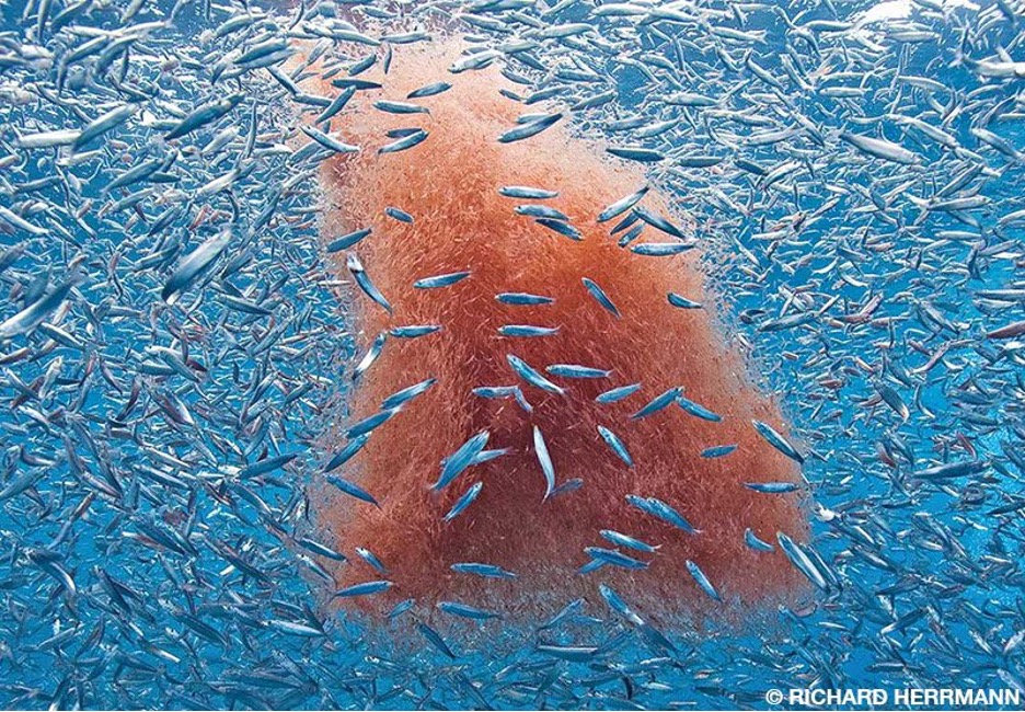
One reason why krill are such advantageous prey type for baleen whales is their tendency to aggregate into dense swarms that may contain hundreds of thousands of individuals. The large body size of baleen whales requires them to feed on such profitable patches (Benoit-Bird, 2024). The packing density of krill within aggregations determines how many a whale can capture in one mouthful, and drives patch selection, such as for blue whales in Antarctica (Miller 2019).
Figure 2. The dense swarms formed by krill make them a prime target for many predators, including these juvenile Pacific sardines. (Photo: Richard Herrmann)
However, even the juiciest, densest krill won’t benefit a foraging whale if the energy required to consume it outweighs the gains. The depth of krill in the water column shapes the acrobatic foraging maneuvers blue whales use to feed (Goldbogen et al., 2015), and is a key driver of patch selection (Miller et al., 2019). The horizontal distance between the whale and a new krill patch is important too. Foraging humpback whales adapt their movements to the hierarchical structure of the preyfield, and feeding on neighboring prey schools can reduce the energy and time expended during interpatch travel, increasing net foraging gain (Kirchner et al., 2018).
Prey quality is dynamic, shaped by environmental conditions, extreme events, and climate change processes (Gomes et al., 2024). We can’t yet fully predict how change will alter prey and predator relationships in the NCC region (Muhling et al., 2020), making every step toward understanding prey dynamics relative to environmental variability key to anticipating how whales will fare in an unknown future (Hildebrand et al., 2021). If you are what you eat, then learning more about krill prey quality will give us unique insights into the baleen whales that come from far and wide to the NCC foraging grounds.
References
Benoit-Bird, K. J. (2024). Resource Patchiness as a Resolution to the Food Paradox in the Sea. The American Naturalist, 203(1), 1–13. https://doi.org/10.1086/727473
Cade, D. E., Kahane-Rapport, S. R., Wallis, B., Goldbogen, J. A., & Friedlaender, A. S. (2022). Evidence for Size-Selective Predation by Antarctic Humpback Whales. Frontiers in Marine Science, 9, 747788. https://doi.org/10.3389/fmars.2022.747788
Fiedler, P. C., Reilly, S. B., Hewitt, R. P., Demer, D., Philbrick, V. A., Smith, S., Armstrong, W., Croll, D. A., Tershy, B. R., & Mate, B. R. (1998). Blue whale habitat and prey in the California Channel Islands. Deep Sea Research Part II: Topical Studies in Oceanography, 45(8–9), 1781–1801. https://doi.org/10.1016/S0967-0645(98)80017-9
Fisher, J. L., Menkel, J., Copeman, L., Shaw, C. T., Feinberg, L. R., & Peterson, W. T. (2020). Comparison of condition metrics and lipid content between Euphausia pacifica and Thysanoessa spinifera in the northern California Current, USA. Progress in Oceanography, 188. https://doi.org/10.1016/j.pocean.2020.102417
Goldbogen, J. A., Hazen, E. L., Friedlaender, A. S., Calambokidis, J., DeRuiter, S. L., Stimpert, A. K., & Southall, B. L. (2015). Prey density and distribution drive the three‐dimensional foraging strategies of the largest filter feeder. Functional Ecology, 29(7), 951–961. https://doi.org/10.1111/1365-2435.12395
Gomes, D. G. E., Ruzicka, J. J., Crozier, L. G., Huff, D. D., Brodeur, R. D., & Stewart, J. D. (2024). Marine heatwaves disrupt ecosystem structure and function via altered food webs and energy flux. Nature Communications, 15(1), 1988. https://doi.org/10.1038/s41467-024-46263-2
Hildebrand, L., Bernard, K. S., & Torres, L. G. (2021). Do Gray Whales Count Calories? Comparing Energetic Values of Gray Whale Prey Across Two Different Feeding Grounds in the Eastern North Pacific. Frontiers in Marine Science, 8. https://doi.org/10.3389/fmars.2021.683634
Kirchner, T., Wiley, D., Hazen, E., Parks, S., Torres, L., & Friedlaender, A. (2018). Hierarchical foraging movement of humpback whales relative to the structure of their prey. Marine Ecology Progress Series, 607, 237–250. https://doi.org/10.3354/meps12789
Miller, E. J., Potts, J. M., Cox, M. J., Miller, B. S., Calderan, S., Leaper, R., Olson, P. A., O’Driscoll, R. L., & Double, M. C. (2019). The characteristics of krill swarms in relation to aggregating Antarctic blue whales. Scientific Reports, 9(1), 16487. https://doi.org/10.1038/s41598-019-52792-4
Muhling, B. A., Brodie, S., Smith, J. A., Tommasi, D., Gaitan, C. F., Hazen, E. L., Jacox, M. G., Auth, T. D., & Brodeur, R. D. (2020). Predictability of Species Distributions Deteriorates Under Novel Environmental Conditions in the California Current System. Frontiers in Marine Science, 7. https://doi.org/10.3389/fmars.2020.00589
Robertson, R. R., & Bjorkstedt, E. P. (2020). Climate-driven variability in Euphausia pacifica size distributions off northern California. Progress in Oceanography, 188. https://doi.org/10.1016/j.pocean.2020.102412
Savoca, M. S., Czapanskiy, M. F., Kahane-Rapport, S. R., Gough, W. T., Fahlbusch, J. A., Bierlich, K. C., Segre, P. S., Di Clemente, J., Penry, G. S., Wiley, D. N., Calambokidis, J., Nowacek, D. P., Johnston, D. W., Pyenson, N. D., Friedlaender, A. S., Hazen, E. L., & Goldbogen, J. A. (2021). Baleen whale prey consumption based on high-resolution foraging measurements. Nature, 599(7883), 85–90. https://doi.org/10.1038/s41586-021-03991-5
Spitz, J., Trites, A. W., Becquet, V., Brind’Amour, A., Cherel, Y., Galois, R., & Ridoux, V. (2012). Cost of Living Dictates what Whales, Dolphins and Porpoises Eat: The Importance of Prey Quality on Predator Foraging Strategies. PLoS ONE, 7(11), e50096. https://doi.org/10.1371/journal.pone.0050096
Videsen, S. K. A., Simon, M., Christiansen, F., Friedlaender, A., Goldbogen, J., Malte, H., Segre, P., Wang, T., Johnson, M., & Madsen, P. T. (2023). Cheap gulp foraging of a giga-predator enables efficient exploitation of sparse prey. Science Advances, 9(25), eade3889. https://doi.org/10.1126/sciadv.ade3889
By Natalie Chazal, PhD student, OSU Department of Fisheries, Wildlife, & Conservation Sciences, Geospatial Ecology of Marine Megafauna Lab
Scientific inquiry relies on quantifying how certain we are of the differences we see in observations. This means that we must look at phenomena based on probabilities that we calculate from observed data, or data that we collect from sampling efforts. Historically, p-values have served as a relatively ubiquitous tool for assessing the strength of evidence in support of a hypothesis. However, as our understanding of statistical methods evolves, so does the scrutiny surrounding the appropriateness and interpretation of p-values. In the realm of research, the debate surrounding the use of p-values for determining statistical significance has sparked some controversy and reflection within the academic community.
What is a p-value?
To understand the debate itself, we need to understand what a p-value is. The p-value represents the probability of obtaining a result as extreme as, or more extreme than, the observed data, under the assumption that there is no true difference or relationship between groups or variables. Traditionally, a p-value below a predetermined threshold (often 0.05) is considered statistically significant, suggesting that the observed data are unlikely (i.e., a 5% probability) to have occurred by chance alone. Many statistical tests provide p-values, which gives us a unified framework for interpretation across a range of analyses.
To illustrate this, imagine a study aimed at investigating the effects of underwater noise pollution on the foraging behavior of gray whales. Researchers collect data on the diving behavior of gray whales in both noisy and quiet regions of the ocean.
Drawings of gray whales with tags (depicted by orange shapes) in quiet areas (left) and noisy areas (right).
In this example, the researchers hypothesize that gray whales stop foraging and ultimately change their diving behavior in response to increased marine noise pollution. The data collected from this hypothetical scenario could come from tags equipped with sensors that record diving depth, duration, and location, allowing us to calculate the exact length of time spent foraging. Data would be collected from both noisy areas (maybe near shipping lanes or industrial sites) and quiet areas (more remote regions with minimal human activity).
To assess the significance of the differences between the two noise regimes, researchers may use statistical tests like t-tests to compare two groups. In our example, researchers use a t-test to compare the average foraging time between whales in noisy and quiet regimes. The next step would be to define hypotheses about the differences we expect to see. The null hypothesis (HN) would be that there is no difference in the average foraging time (X) between noisy and quiet areas:
Scenario where the noisy area does not elicit a behavioral response that can be detected by the data collected by the tags (orange shapes on whales back). The lower graph shows the distribution of the data (foraging time) for the noisy and the quiet areas. The means of this data (X) are not different.
And the alternative hypothesis (HA) would be that there is a difference between the noisy and quiet areas:
Scenario where the noisy area elicits a behavioral response (swimming more towards the surface instead of foraging) that can be detected by the data collected by the tags (orange shapes on whales back). The lower graph shows the distribution of the data (foraging time) for the noisy and the quiet areas. The means of this data (X) are different with the noisy mean foraging time (pink) being lower than the quiet mean foraging time (blue).
For now, we will skip over the nitty gritty of a t-test and just say that the researchers get a “t-score” that says whether or not there is a difference in the means (X) of the quiet and noisy areas. A larger t-score means that there is a difference in the means whereas a smaller t-score would indicate that the means are more similar. This t-score comes along with a p-value. Let’s say we get a t-score (green dot) that is associated with a p-value of 0.03 shown as the yellow area under the curve:
The t-score is a test statistic that tells us how different the means of our observed data groups are from each other (green dot). The area under the t-distribution that is above the t-score is the p-value (yellow shaded area).
A p-value of 0.03 means that there is a 3% probability of obtaining these observed differences in foraging time between noisy and quiet areas purely by chance, which assumes that the null hypothesis is true (that there is no difference). We usually compare this p-value to a threshold value to say whether this finding is significant. We set this threshold before looking at the results of the test. If the threshold is above our value, like 0.05, then we can “reject the null hypothesis” and conclude that there is a significant difference in foraging time between noisy and quiet areas (green check mark scenario). On the flip-side, if the threshold that we set before our results is too low (0.01), then we will “fail to reject the null hypothesis” and conclude that there was no significant difference in foraging time between noisy and quiet areas (red check mark scenario). The reason that we don’t ever “accept the null” is because we are testing an alternative hypothesis with observations and if those observations are consistent with the null rather than the alternative, this is not evidence for the null because it could be consistent with a different alternative hypothesis that we are not yet testing for.
When our pre-set threshold to determine significance is above or greater than our p-value that was calculated we have enough evidence to ‘reject the null hypothesis’ (left figure) whereas if our p-value is lower or smaller than our calculated p-value, then we ‘fail to reject the null hypothesis’ (right figure).
In this example, the use of p-values helps the researchers quantify the strength of evidence for their hypothesis and determine whether the observed differences in gray whale behavior are likely to be meaningful or merely due to chance.
The Debate
Despite its widespread use, the reliance on p-values has been met with criticism. Firstly, because p-values are so ubiquitous, it can be easy to calculate them with or without enough critical thinking or interpretation. This critical thinking should include an understanding of what is biologically relevant and avoid the trap of using binary language like significant or non-significant results instead of looking directly at the uncertainty of your results. One of the other most common misconceptions about p-values is that they can measure the direct probability of the null hypothesis being true. As amazing as that would be, in reality we can only use p-values to understand the probability of our observed data. Additionally, it’s common to conflate the significance or magnitude of the p-value with effect size (which is the strength of the relationship between the variables). You can have a small p-value for an effect that isn’t very large or meaningful, especially if you have a large sample size. Sample size is an important metric to report. Larger number of samples generally means more precise estimates, higher statistical power, increased generalizability, and higher possibility for replication.
Furthermore, in studies that require multiple comparisons (i.e. multiple statistical analyses are done in a single study), there is an increased likelihood of observing false positives because each test introduces a chance of obtaining a significant result by random variability alone. In p-value language, a “false positive” is when you say something is significant (below your p-value threshold) when it actually is not, and a “false negative” is when you say something is not significant (above the p-value threshold) when it actually is. So, in terms of multiple comparisons, if there are no adjustments made for the increased risk of false positives, this can potentially lead to inaccurate conclusions of significance.
In our example using foraging time in gray whales, we didn’t consider the context of our findings. To make this a more reliable study, we have to consider factors like the number of whales tagged (sample size!), the magnitude of noise near the tagged whales, other variables in the environment (e.g. prey availability) that could affect our results, and the ecological significance in the difference in foraging time that was found. To make robust conclusions, we need to carefully build hypotheses and study designs that will answer the questions we seek. We must then carefully choose the statistical tests that we use and explore how our data align with the assumptions that these tests make. It’s essential to contextualize our results within the bounds of our study design and broader ecological system. Finally, performing sensitivity analyses (e.g. running the same tests multiple times on slightly different datasets) ensures that our results are stable over a variety of different model parameters and assumptions.
In the real world, there have been many studies done on the effects of noise pollution on baleen whale behavior that incorporate multiple sources of variance and bias to get robust results that show behavioral responses and physiological consequences to anthropogenic sound stressors (Melcón et al. 2012, Blair et al. 2016, Gailey et al. 2022, Lemos et al. 2022).
Moving Beyond P-values
There has been growing interest in reassessing the role of p-values in scientific inference and publishing. Scientists appreciate p-values because they provide one clear numeric threshold to determine significance of their results. However, the reality is more complicated than this binary approach. We have to explore the uncertainty around these estimates and test statistics (e.g. t-score) and what they represent ecologically. One avenue to explore might be focusing more on effect sizes and confidence intervals as more informative measures of the magnitude and precision of observed effects. There has also been a shift towards using Bayesian methods, which allow for the incorporation of prior knowledge and a more nuanced quantification of uncertainty.
Bayesian methods in particular are a leading alternative to p-values because instead of looking at how likely our observations are given a null hypothesis, we get a direct probability of the hypothesis given our data. For example, we can use Bayes factor for our noisy vs quiet gray whale behavioral t-test (Johnson et al. 2023). Bayes factor measures the likelihood of the data being observed for each hypothesis separately (instead of assuming the null hypothesis is true) so if we calculate a Bayes factor of 3 for the alternative hypothesis (HA), we could directly say that it is 3 times more likely for there to be decreased foraging time in a noisy area than for there to be no difference in the noisy vs quiet group. But that is just one example of Bayesian methods at work. The GEMM lab uses Bayesian methods in many projects from Lisa’s spatial capture-recapture models (link to blog) and Dawn’s blue whale abundance estimates (Barlow et al. 2018) to quantifying uncertainty associated with drone photogrammetry data collection methods in KC’s body size models (link to blog).
Ultimately, the debate surrounding p-values highlights the necessity of nuanced and transparent approaches to statistical inference in scientific research. Rather than relying solely on arbitrary thresholds, researchers can consider the context, relevance, and robustness of their findings. From justifying our significance thresholds to directly describing parameters based on probability, we have increasingly powerful tools to improve the methodological rigor of our studies.
Barlow, D.R., Torres, L.G., Hodge, K.B., Steel, D., Baker, C.S., Chandler, T.E., Bott, N., Constantine, R., Double, M.C., Gill, P., Glasgow, D., Hamner, R.M., Lilley, C., Ogle, M., Olson, P.A., Peters, C., Stockin, K.A., Tessaglia-Hymes, C.T., Klinck, H., 2018. Documentation of a New Zealand blue whale population based on multiple lines of evidence. Endangered Species Research 36, 27–40. https://doi.org/10.3354/esr00891
Blair, H.B., Merchant, N.D., Friedlaender, A.S., Wiley, D.N., Parks, S.E., 2016. Evidence for ship noise impacts on humpback whale foraging behaviour. Biol Lett 12, 20160005. https://doi.org/10.1098/rsbl.2016.0005
Gailey, G., Sychenko, O., Zykov, M., Rutenko, A., Blanchard, A., Melton, R.H., 2022. Western gray whale behavioral response to seismic surveys during their foraging season. Environ Monit Assess 194, 740. https://doi.org/10.1007/s10661-022-10023-w
Halsey, L.G., 2019. The reign of the p-value is over: what alternative analyses could we employ to fill the power vacuum? Biology Letters 15, 20190174. https://doi.org/10.1098/rsbl.2019.0174
Johnson, V.E., Pramanik, S., Shudde, R., 2023. Bayes factor functions for reporting outcomes of hypothesis tests. Proceedings of the National Academy of Sciences 120, e2217331120. https://doi.org/10.1073/pnas.2217331120
Lemos, L.S., Haxel, J.H., Olsen, A., Burnett, J.D., Smith, A., Chandler, T.E., Nieukirk, S.L., Larson, S.E., Hunt, K.E., Torres, L.G., 2022. Effects of vessel traffic and ocean noise on gray whale stress hormones. Sci Rep 12, 18580. https://doi.org/10.1038/s41598-022-14510-5
Dr. Alejandro A. Fernández Ajó, Postdoctoral Scholar, Marine Mammal Institute – OSU Department of Fisheries, Wildlife, & Conservation Sciences, Geospatial Ecology of Marine Megafauna (GEMM) Lab.
The Eastern North Pacific (ENP) gray whale population has experienced at least two recorded Unusual Mortality Events (UMEs), from 1999–2000 and from 2019 to 2024, during which many gray whales stranded along the Pacific coast from northern Mexico to the Alaskan Arctic, USA (Martínez-Aguilar et al., 2019; Urbán, 2020). Several factors have been considered as possible causes for the high number of gray whale’s strandings, including variation in Arctic prey availability and the duration of their feeding season caused by the timing of sea ice formation and breakup (Stewart et al., 2023), starvation, anthropogenically derived toxicants, biotoxins, infectious diseases, parasites, fisheries interactions, and ship strikes (F. Gulland et al., 2005). In the most recent UME, many of the stranded whales showed signs of emaciation, indicating malnutrition as a causal factor of death (Christiansen et al., 2021; Torres et al., 2022). While the poor condition of many of the stranded whales supports the idea of starvation as a cause for these mortalities, the underlying causes of malnutrition are unknown, and it is also unclear whether the whales’ decline in body condition was rapid or gradual.
Large whales face a multitude of stressors in their environment, ranging from ocean noise to contaminants, climate change, and prey shifts. Understanding how individual whales respond to these disturbances is crucial for assessing potential impacts on the population as a whole. However, monitoring the health parameters and vital rates of whales presents significant challenges due to their large size, mobility, and the vast ranges of their marine habitat. Studying stranded whales can provide valuable insights into health risks, disease susceptibility, and the impacts of pollutants and other stressors on whale populations, thus informing conservation strategies (see post). Nonetheless, the quality of information obtained from necropsies heavily relies on the timeliness of stranding reports, as decomposition begins immediately after death, limiting detailed investigations into the cause of death. Therefore, establishing a robust network capable of promptly reporting and addressing stranding events is essential (Gulland & Stockin, 2020). An effective network involves having well-trained staff, proper infrastructure, sufficient funding, and the expertise and tools necessary to gather and analyze data and samples to infer their health and causes of mortality.
During my doctoral dissertation, I worked to develop and ground truth the endocrine analyses of whale baleen as a novel sample type that can be used for retrospective assessments of the whale’s physiology (see my previous post & post). Baleen, the filter-feeding apparatus of mysticetes whales (Figure 1), consists of long fringed plates of keratinized tissue that grow continuously and slowly downward from the whale’s upper jaw. These plates are routinely collected at necropsies; and unlike other tissue types, they are durable and have minimum storage requirements; they can be preserved dry at room temperature, allowing for the analysis of both historical and current whale populations. Moreover, while most sample types used for studying whale health and physiology provide a single time-point measure of current circulating hormone levels (e.g., skin or respiratory vapor) or hold integrated information from the previous few hours or days (e.g., urine and feces), baleen tissue provides a unique opportunity for retrospective and longitudinal analyses of multiple biological parameters of the individual during the time that the tissue was grown, i.e., months to years prior to death, helping to describe the whale’s physiology, migration patterns, and exposure to pollutants (see my previous post).
In our recent study, “A longitudinal study of endocrinology and foraging ecology of subadult gray whales prior to death based on baleen analysis”, published in the journal General and Comparative Endocrinology, we examine isotope and hormone levels in the baleen of five young gray whales stranded in central Oregon during the most recent UME. Our primary objectives were to retrospectively examine the hormone and isotopic profiles of the individual whales prior to mortality, assess potential factors contributing to death, and identify the timing for the onset of chronic illness leading to mortality. Our analysis included tracing longitudinal changes in (1) stable isotope values in baleen (δ13C and δ15N), which allowed us to infer the baleen growth rate and assess the seasonal changes in diet and foraging location in large whales (Figure 2), along with the quantification of (2) two adrenal glucocorticoid steroids that are biomarkers for the whale’s stress response, (3) one thyroid hormone (triiodothyronine, T3) as an indicator of nutritional state, and (4) two sex hormones, progesterone and testosterone, to infer about reproductive status and sexual maturity. By integrating isotopic and hormonal methodologies, our study demonstrates how baleen analysis offers a comprehensive narrative of the endocrine and trophic ecology of individual whales over time.
Figure 2. Gray whales, like other large marine mammals that rely on built-up energy reserves, exhibit distinct seasonal shifts in their feeding habits. During summer, these whales feed at the ocean’s bottom, consuming organisms lower in the food chain, which is reflected in lower nitrogen values in their baleen (summer foraging). In winter, however, they must rely on their own fat reserves, causing an increase in nitrogen values (wintering). In this plot we can observe the oscillations in δ15N over time; this information allows us to estimate the baleen growth rate. Our results suggest that gray whale baleen holds a record of around 1.3 years of stable isotopes and hormone data prior to the time of death (Fernandez Ajo et al. 2024). The red cross in the X-axis, indicate the time of death. Gray whale illustration https://www.fisheries.noaa.gov/species/gray-whale
Our endocrine assessments revealed detailed profiles of stress-related hormones (glucocorticoids, cortisol) and thyroid hormones along the lengths of the baleen. We found increased levels of cortisol in whales that died from unknown causes, starting about eight months prior to their deaths. This suggests these whales were under prolonged stress before dying. In contrast, in the case of a whale killed acutely by a killer whale, cortisol levels were low and constant prior to death, indicating this individual was likely in good health prior to the sudden attack. In terms of thyroid activity, indicated by T3 hormone levels, we found a gradual increase over several months in the whales that died of unknown causes. This pattern is not typically expected, as stress usually suppresses thyroid function. This anomaly could suggest an adaptive response to maintain body temperature and metabolism in potentially malnourished whales. Regarding the sex hormones, as expected for this age class, we found no significant fluctuations or spikes that would indicate sexual maturity in these young whales (Figure 3).
Figure 3. Longitudinal hormone profiles in an individual gray whale that died due to unknown causes (left) and one that died acutely due to orca predation (right). Note the pronounced elevations in cortisol levels (indicative of stress) and T3 prior to death in the case of unknown cause of death, while hormone levels remained low and constant prior to death in the whale acutely killed. Sex hormones do not present any clear oscillations, indicating that these whales were likely sexually immature. The red cross in the X-axis, indicate the time of death. Killer whale (Orcinus orca) illustration https://www.fisheries.noaa.gov/species/killer-whale
Although commercial whaling is currently banned and several whale populations show evidence of recovery, today’s whales are exposed to a variety of other human stressors that cause significant lethal and non-lethal impacts (e.g., entanglement in fishing gear, vessel strikes, shipping noise, climate change, etc.; reviewed in Thomas et al., 2016). The recovery and conservation of large whale populations is particularly important to the oceanic environment due to their key ecological role and unique biological traits (See my previous post). Our research demonstrates the strengths of using baleen as a tool for the retrospective assessments of whale endocrinology and trophic ecology. As the Eastern North Pacific gray whale population faces recurring challenges, indicated by fluctuating numbers and unusual mortality events, innovative techniques like the baleen analysis presented here, are essential to investigate the causes of mortality and inform management, helping us understand not only the immediate causes of death but also broader environmental and ecological changes affecting their survival. Broadly implementing this approach with a greater sample size of baleen collected across a larger spatial and temporal range could significantly improve our strategies for conservation and management of baleen whales.
Did you enjoy this blog? Want to learn more about marine life, research, and conservation? Subscribe to our blog and get a weekly message when we post a new blog. Just add your name and email into the subscribe box below.
References
Christiansen, F., Rodríguez-González, F., Martínez-Aguilar, S., Urbán, J., Swartz, S., Warick, H., Vivier, F., & Bejder, L. (2021). Poor body condition associated with an unusual mortality event in gray whales. Marine Ecology Progress Series, 658, 237–252. https://doi.org/10.3354/meps13585
Gulland, F. M. D., & Stockin, K. A. (2020). Harmonizing global strandings response. European Cetacean Society Special Publication Series.
Gulland, F., Pérez-Cortés, H., Urbán, J. R., Rojas-Bracho, L., Ylitalo, G., Weir, J., Norman, S., Muto, M., Rugh, D., Kreuder, C., & Rowles, T. (2005). Eastern North Pacific gray whale (Eschrichtius robustus) unusual mortality event, 1999-2000. U.S. Department of Commerce. NOAA Technical Memorandum. NMFS-AFSC-150., March, 33 pp. http://www.afsc.noaa.gov/publications/AFSC-TM/NOAA-TM-AFSC-150.pdf
Martínez-Aguilar, S., Mariano-Meléndez, E., López-Paz, N., Castillo-Romero, F., Zaragoza-aguilar, G. A., Rivera-Rodriguez, J., Zaragoza-Aguilar, A., Swartz, S., Viloria-Gómora, L., & Urbán, J. R. (2019). Gray whale (Eschrichtius robustus) stranding records in Mexico during the winter breeding season in 2019. Report of the International Whaling Commission. Document SC/68A/CMP/14, May.
Stewart, J. D., Joyce, T. W., Durban, J. W., Calambokidis, J., Fauquier, D., Fearnbach, H., Grebmeier, J. M., Lynn, M., Manizza, M., Perryman, W. L., Tinker, M. T., & Weller, D. W. (2023). Boom-bust cycles in gray whales associated with dynamic and changing Arctic conditions. Science, 382(6667), 207–211. https://doi.org/10.1126/science.adi1847
Torres, L. G., Bird, C. N., Rodríguez-González, F., Christiansen, F., Bejder, L., Lemos, L., Urban R, J., Swartz, S., Willoughby, A., Hewitt, J., & Bierlich, KC. (2022). Range-Wide Comparison of Gray Whale Body Condition Reveals Contrasting Sub-Population Health Characteristics and Vulnerability to Environmental Change. Frontiers in Marine Science, 9. https://doi.org/10.3389/fmars.2022.867258
Urbán, R. (2020). Gray whale stranding records in Mexico during the 2020 winter breeding season. Unpublished Paper SC/68B/CMP/13 Presented to the IWC Scientific Committee, Cambridge.