Clara Bird, PhD Student, OSU Department of Fisheries, Wildlife, and Conservation Sciences, Geospatial Ecology of Marine Megafauna Lab
“Why don’t you just automate it?” This is a question I am frequently asked when I tell someone about my work. My thesis involves watching many hours of drone footage of gray whales and meticulously coding behaviors, and there are plenty of days when I have asked myself that very same question. Streamlining my process is certainly appealing and given how wide-spread and effective machine learning methods have become, it is a tempting option to pursue. That said, machine learning is only appropriate for certain research questions and scales, and it’s important to consider these before investing in using a new tool.
The application of machine learning methods to behavioral ecology is called computational ethology (Anderson & Perona, 2014). To identify behaviors from videos, the model tracks individuals across video frames and identifies patterns of movement that form a behavior. This concept is similar to the way we identify a whale as traveling if it’s moving in a straight line and as foraging if it’s swimming in circles within a small area (Mayo & Marx, 1990, check out this blog to learn more). The level of behavioral detail that the model is able to track depends on the chosen method (Figure 1, Pereira et al., 2020). These methods range from tracking each animal as a simple single point (called a centroid) to tracking the animal’s body positioning in 3D (this method is called pose estimation), which range from providing less detailed to more detailed behavior definitions. For example, tracking an individual as a centroid could be used to classify traveling and foraging behaviors, while pose estimation could identify specific foraging tactics.

Pose estimation involves training the machine learning algorithm to track individual anatomical features of an individual (e.g., the head, legs, and tail of a rat), meaning that it can define behaviors in great detail. A behavior state could be defined as a combination of the angle between the tail and the head, and the stride length.
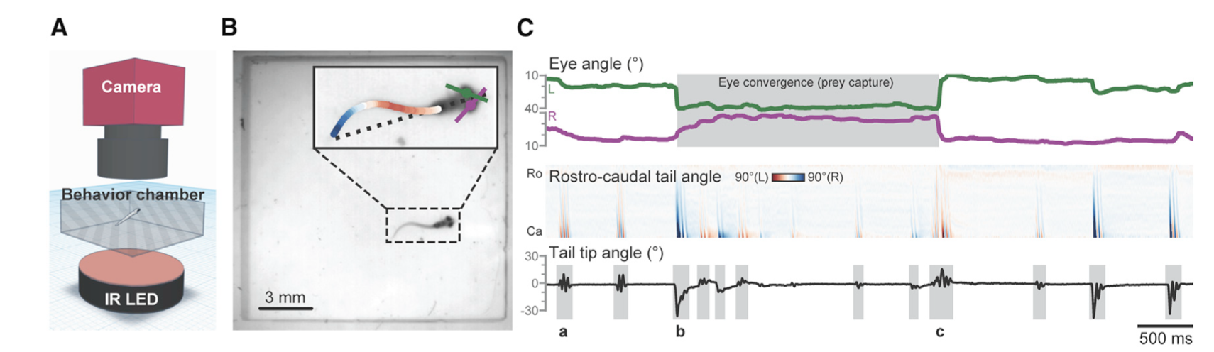
For example, Mearns et al. (2020) used pose estimation to study how zebrafish larvae in a lab captured their prey. They tracked the tail movements of individual larvae when presented with prey and classified these movements into separate behaviors that allowed them to associate specific behaviors with prey capture (Figure 2). The authors found that these behaviors occurred in a specific sequence, that the behaviors kept the prey within the larvae’s line of sight, and that the sequence was triggered by visual cues. In fact, when they removed the visual cue of the prey, the larvae terminated the behavior sequence, meaning that the larvae are continually choosing to do each behavior in the sequence, rather than the sequence being one long behavior event that is triggered only by the initial visual cue. This study is a good example of the applicability of machine learning models for questions aimed at kinematics and fine-scale movements. Pose estimation has also been used to study the role of facial expression and body language in rat social communication (Ebbesen & Froemke, 2021).
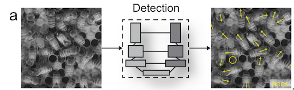
While previous machine learning methods to track animal movements required individuals to be physically marked, the current methods can perform markerless tracking (Pereira et al., 2020). This improvement has broadened the kinds of studies that are possible. For example, Bozek et al., (2021) developed a model that tracked individuals throughout an entire honeybee colony and showed that certain individual behaviors were spatially distributed within the colony (Figure 3). Machine learning enabled the researchers to track over 1000 individual bees over several months, a task that would be infeasible for someone to do by hand.
These studies highlight that the potential benefits of using machine learning when studying fine scale behaviors (like kinematics) or when tracking large groups of individuals. Furthermore, once it’s trained, the model can process large quantities of data in a standardized way to free up time for the scientists to focus on other tasks.
While machine learning is an exciting and enticing tool, automating behavior detection via machine learning could be its own PhD dissertation. Like most things in life, there are costs and benefits to using this technique. It is a technically difficult tool, and while applications exist to make it more accessible, knowledge of the computer science behind it is necessary to apply it effectively and correctly. Secondly, it can be tedious and time consuming to create a training dataset for the model to “learn” what each behavior looks like, as this step involves manually labeling examples for the model to use.
As I’ve mentioned in a previous blog, I came quite close to trying to study the kinematics of gray whale foraging behaviors but ultimately decided that counting fluke beats wasn’t necessary to answer my behavioral research questions. It was important to consider the scale of my questions (as described in Allison’s blog) and I think that diving into more fine-scale kinematics questions could be a fascinating follow-up to the questions I’m asking in my PhD.
For instance, it would be interesting to quantify how gray whales use their flukes for different behavior tactics. Do gray whales in better body condition beat their flukes more frequently while headstanding? Does the size of the fluke affect how efficiently they can perform certain tactics? While these analyses would help quantify the energetic costs of different behaviors in better detail, they aren’t necessary for my broad scale questions. Consequently, taking the time to develop and train a pose estimation machine learning model is not the best use of my time.
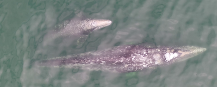
That being said, I am interested in applying machine learning methods to a specific subset of my dataset. In social behavior, it is not only useful to quantify the behaviors exhibited by each individual but also the distance between them. For example, the distance between a mom and her calf can be indicative of the calves’ dependence on its mom (Nielsen et al., 2019). However, continuously measuring the distance between two individuals throughout a video is tedious and time intensive, so training a machine learning model could be an effective use of time. I plan to work with an intern this summer to develop a machine learning model to track the distance between pairs of gray whales in our drone footage and then relate this distance data with the manually coded behaviors to examine patterns in social behavior (Figure 4). Stay tuned to learn more about our progress!
Did you enjoy this blog? Want to learn more about marine life, research, and conservation? Subscribe to our blog and get a weekly alert when we make a new post! Just add your name into the subscribe box on the left panel.
References
Anderson, D. J., & Perona, P. (2014). Toward a Science of Computational Ethology. Neuron, 84(1), 18–31. https://doi.org/10.1016/j.neuron.2014.09.005
Bozek, K., Hebert, L., Portugal, Y., Mikheyev, A. S., & Stephens, G. J. (2021). Markerless tracking of an entire honey bee colony. Nature Communications, 12(1), 1733. https://doi.org/10.1038/s41467-021-21769-1
Ebbesen, C. L., & Froemke, R. C. (2021). Body language signals for rodent social communication. Current Opinion in Neurobiology, 68, 91–106. https://doi.org/10.1016/j.conb.2021.01.008
Mayo, C. A., & Marx, M. K. (1990). Surface foraging behaviour of the North Atlantic right whale, Eubalaena glacialis , and associated zooplankton characteristics. Canadian Journal of Zoology, 68(10), 2214–2220. https://doi.org/10.1139/z90-308
Mearns, D. S., Donovan, J. C., Fernandes, A. M., Semmelhack, J. L., & Baier, H. (2020). Deconstructing Hunting Behavior Reveals a Tightly Coupled Stimulus-Response Loop. Current Biology, 30(1), 54-69.e9. https://doi.org/10.1016/j.cub.2019.11.022
Nielsen, M., Sprogis, K., Bejder, L., Madsen, P., & Christiansen, F. (2019). Behavioural development in southern right whale calves. Marine Ecology Progress Series, 629, 219–234. https://doi.org/10.3354/meps13125
Pereira, T. D., Shaevitz, J. W., & Murthy, M. (2020). Quantifying behavior to understand the brain. Nature Neuroscience, 23(12), 1537–1549. https://doi.org/10.1038/s41593-020-00734-z


