By Matoska Silva, OSU Department of Integrative Biology, CEOAS REU Program
My name is Matoska Silva, and I just finished my first year at Oregon State University studying biology with a focus in ecology. This summer will be my first experience with marine ecology, and I’m eager to dive right in. I’m super excited for the opportunity to research krill due to the huge impacts these tiny organisms have on their surrounding ecosystems. The two weeks I’ve spent in the CEOAS REU so far have been among the most fun and informative of my life, and I can’t wait to see what else the summer has in store for me.

I’ve spent most of my life in Oregon, so I was thrilled to learn that my project would focus on krill distribution along the Oregon Coast that I know and love. More specifically, my project focuses on the Northern California Current (NCC, the current found along the Oregon Coast) and the ways that geographic distribution of krill corresponds to climatic conditions in the region. Here is a synopsis of the project:
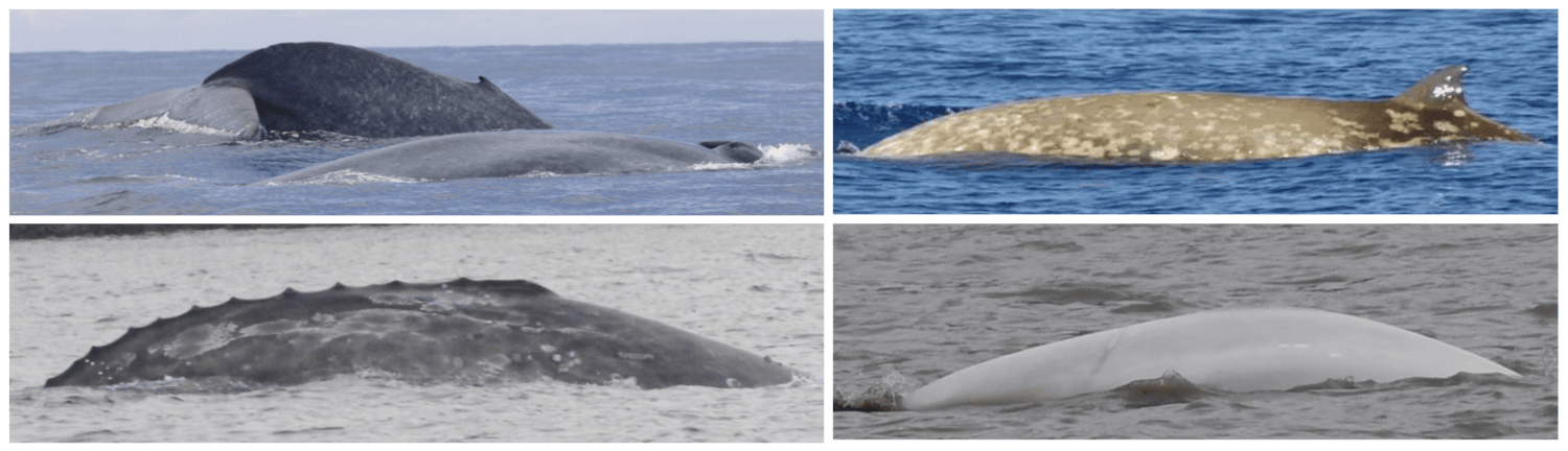
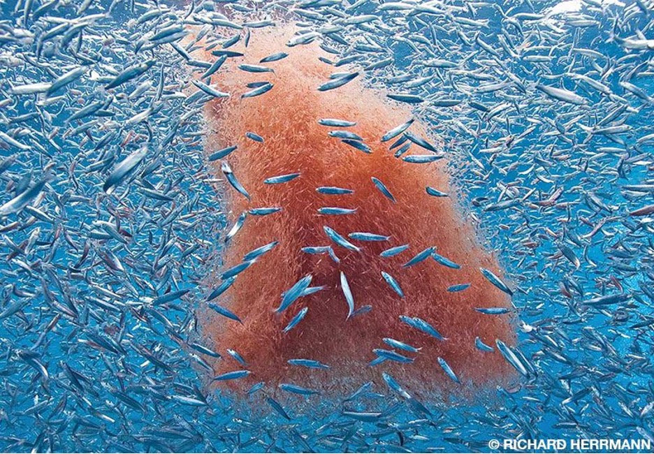
The NCC system, which spans the west coast of North America from Cape Mendocino, California to southern British Columbia, is notable for seasonal upwelling, a process that brings cool, nutrient-rich water from the ocean depths to the surface. This process provides nutrients for a complex marine food web containing phytoplankton, zooplankton, fish, birds, and mammals (Checkley & Barth, 2009). Euphausiids, commonly known as krill, are among the most ecologically important zooplankton groups in the NCC, playing a vital role in the flow of nutrients through the food web (Evans et al., 2022). Euphausia pacifica and Thysanoessa spinifera are the predominant krill species in the NCC, with T. spinifera mainly inhabiting coastal waters and E. pacifica inhabiting a wider range offshore (Brinton, 1962). T. spinifera individuals are typically physically larger than E. pacifica and are generally a higher-energy food source for predators (Fisher et al., 2020).
Temperature has been previously established as a major factor impacting krill abundance and distribution in the NCC (Phillips et al., 2022). Massive, ecosystem-wide changes in the NCC have been linked to extreme warming brought on by the 2014-2016 marine heatwave (Brodeur et al., 2019). Both dominant krill species have been shown to respond negatively to warming events in the NCC, with anomalous warm temperatures in 2014-2016 being linked to severe declines in E. pacifica biomass and with T. spinifera nearly disappearing from the Oregon Coast (Peterson et al., 2017). Changes in normal seasonal size variation and trends toward smaller size distributions in multiple age groups have been observed in E. pacifica in response to warming in northern California coastal waters (Robertson & Bjorkstedt, 2020).
The El Niño-Southern Oscillation (ENSO) is a worldwide climatic pattern that has been linked to warming events and ecosystem disturbances in the California Current System (McGowan et al., 1998). El Niño events of both strong and weak intensity can result in changes in the NCC ecosystem (Fisher et al., 2015). Alterations in the typical zooplankton community accompanying warm water conditions and a decline in phytoplankton have been recorded in the NCC during weak and strong El Niño occurrences (Fisher et al., 2015). A strong El Niño event occurred in 2023 and 2024, with three-month Oceanic Niño Index means reaching above 1.90 from October 2023 to January 2024 (NOAA Climate Prediction Center, https://www.cpc.ncep.noaa.gov/data/indices/oni.ascii.txt).

While patterns in krill responses to warming have been described from previous years, the effects of the 2023-2024 El Niño on the spatial distribution of krill off the Oregon coast have not yet been established. As climate models have predicted that strong El Niño events may become more common due to greenhouse warming effects (Cai et al., 2014), continuing efforts to document zooplankton responses to El Niño conditions are vital for understanding how the NCC ecosystem responds to a changing climate. By investigating krill spatial distributions in April 2023, during a period of neutral ENSO conditions following a year of La Niña conditions, and April 2024, during the 2023-2024 El Niño event, we can assess how recent ENSO activity has impacted krill distributions in the NCC. In addition to broader measures of ENSO, we will examine records of localized sea surface temperatures (SST) and measurements of upwelling activity during April 2023 and 2024.
Understanding spatial distribution of krill aggregations is both ecologically and economically relevant, with implications for both marine conservation and management of commercial fisheries. Modeling patterns in the distribution of krill species and their predators has potential to inform marine management decisions to mitigate human impacts on marine mammals like whales (Rockwood et al., 2020). The data used to identify krill distribution were originally collected as part of the Marine Offshore Species Assessments to Inform Clean Energy (MOSAIC) project. The larger MOSAIC initiative centers around monitoring marine mammals and birds in areas identified for possible future development of offshore wind energy infrastructure. The findings of this study could aid in the conservation of krill consumers during the implementation of wind energy expansion projects. Changes in krill spatial distribution are also important for monitoring species that support commercial fisheries. Temperature has been shown to play a role in the overlap in distribution of NCC krill and Pacific hake (Merluccius productus), a commercially valuable fish species in Oregon waters (Phillips et al., 2023). The findings of my project could supplement existing commercial fish abundance surveys by providing ecological insights into factors driving changes in economically important fisheries.

I’m very grateful for the chance to work on a project with such important implications for the future of our Oregon coast ecosystems. My project has a lot of room for additional investigation of climate variables, with limited time being the main constraint on which processes I can explore. There are also unique methodological challenges to address during the project, and I’m ready to do some experimentation to work out solutions. Wherever my project takes me, I know that I will have developed a diverse range of skills and knowledge of krill by the end of the summer.
References
Brinton, E. (1962). The distribution of Pacific euphausiids. Bulletin of the Scripps Institution of Oceanography, 8(2), 51-270. https://escholarship.org/uc/item/6db5n157
Brodeur, R. D., Auth, T. D., & Phillips, A. J. (2019). Major shifts in pelagic micronekton and macrozooplankton community structure in an upwelling ecosystem related to an unprecedented marine heatwave. Frontiers in Marine Science, 6. https://doi.org/10.3389/fmars.2019.00212
Cai, W., Borlace, S., Lengaigne, M., van Rensch, P., Collins, M., Vecchi, G., Timmermann, A., Santoso, A., McPhaden, M. J., Wu, L., England, M. H., Wang, G., Guilyardi, E., & Jin, F. F. (2014). Increasing frequency of extreme El Niño events due to greenhouse warming. Nature Climate Change, 4, 111–116. https://doi.org/10.1038/nclimate2100
Checkley, D. M., & Barth, J. A. (2009). Patterns and processes in the California Current System. Progress in Oceanography, 83, 49–64. https://doi.org/10.1016/j.pocean.2009.07.028
Evans, R., Gauthier, S., & Robinson, C. L. K. (2022). Ecological considerations for species distribution modelling of euphausiids in the Northeast Pacific Ocean. Canadian Journal of Fisheries and Aquatic Sciences, 79, 518–532. https://doi.org/10.1139/cjfas-2020-0481
Fisher, J. L., Peterson, W. T., & Rykaczewski, R. R. (2015). The impact of El Niño events on the pelagic food chain in the northern California Current. Global Change Biology, 21, 4401–4414. https://doi.org/10.1111/gcb.13054
Fisher, J. L., Menkel, J., Copeman, L., Shaw, C. T., Feinberg, L. R., & Peterson, W. T. (2020). Comparison of condition metrics and lipid content between Euphausia pacifica and Thysanoessa spinifera in the Northern California Current, USA. Progress in Oceanography, 188, 102417. https://doi.org/10.1016/j.pocean.2020.102417
McGowan, J. A., Cayan, D. R., & Dorman, L. M. (1998). Climate-ocean variability and ecosystem response in the Northeast Pacific. Science, 281, 210–217. https://doi.org/10.1126/science.281.5374.210
Phillips, E. M., Chu, D., Gauthier, S., Parker-Stetter, S. L., Shelton, A. O., & Thomas, R. E. (2022). Spatiotemporal variability of Euphausiids in the California Current Ecosystem: Insights from a recently developed time series. ICES Journal of Marine Science, 79, 1312–1326. https://doi.org/10.1093/icesjms/fsac055
Phillips, E. M., Malick, M. J., Gauthier, S., Haltuch, M. A., Hunsicker, M. E., Parker‐Stetter, S. L., & Thomas, R. E. (2023). The influence of temperature on Pacific hake co‐occurrence with euphausiids in the California Current Ecosystem. Fisheries Oceanography, 32, 267–279. https://doi.org/10.1111/fog.12628
Peterson, W. T., Fisher, J. L., Strub, P. T., Du, X., Risien, C., Peterson, J., & Shaw, C. T. (2017). The pelagic ecosystem in the Northern California Current off Oregon during the 2014–2016 warm anomalies within the context of the past 20 years. Journal of Geophysical Research: Oceans, 122(9), 7267–7290. https://doi.org/10.1002/2017jc012952
Robertson, R. R., & Bjorkstedt, E. P. (2020). Climate-driven variability in Euphausia pacificasize distributions off Northern California. Progress in Oceanography, 188, 102412.https://doi.org/10.1016/j.pocean.2020.102412