Dawson Mohney, TOPAZ/JASPER HS Intern, Pacific High School Graduate
My name is Dawson Mohney, I am a high school intern for the 2025 TOPAZ/JASPER team this field season. I first heard about the TOPAZ/JASPER internship from my friend Jonah Lewis, a previous intern from the 2023 field season. Coincidentally, Jonah and I both graduated this year from Pacific High School here on the coast—small world. I have called Port Orford my home for most of my life, and in recent years I discovered that a gray whale research project has been happening in my own backyard. Growing up less than a mile from the Oregon Coast, I’ve spent a lot of time looking out into the water. I always liked how, no matter what happened in my life, the ocean was always there. This interest is what encouraged me to apply for the internship with the hope of discovering more about the ocean, a substantial part of my home and family.
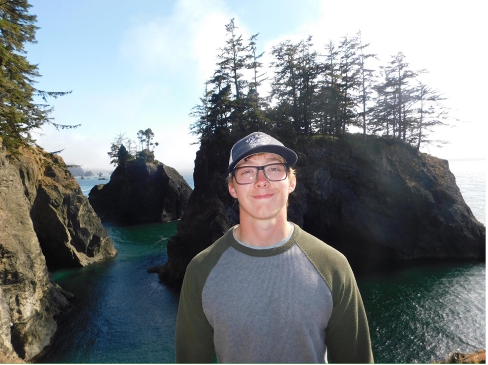
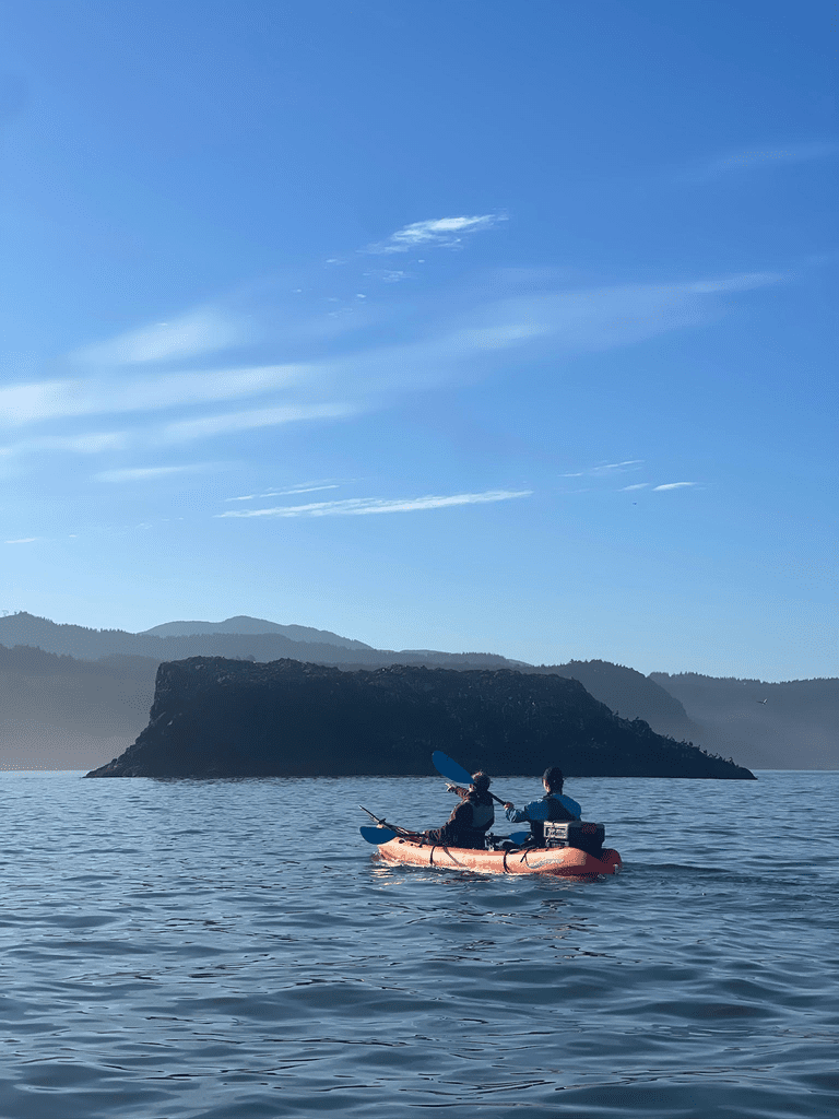
Fig 1: Picture fellow intern Maddie took of me (Dawson) during our trip to Natural Bridges.
A critical part of this project is understanding not only the magnificent gray whales but also the much less apparent zooplankton–after all, the whales need to eat a lot of zooplankton! Many different species of zooplankton—“zoop” for short—call the Oregon coast home. Each day, as we kayak to our 12 sample stations within the gray whale feeding grounds of Mill Rocks and Tichenor’s Cove, I find myself wondering which species of zoop I’ll get to identify later under the microscope.
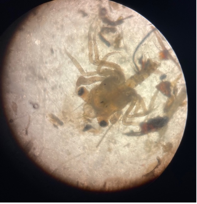
Throughout the duration of this internship, our team has met to discuss a few research papers published by GEMM Lab members, including research produced from the TOPAZ/JASPER projects. Recently, I read, “Do Gray Whales Count Calories? Comparing Energetic Values of Gray Whale Prey Across Two Different Feeding Grounds in the Eastern North Pacific,” by Hildebrand et al. who describe the caloric content of different zooplankton species. Before reading this paper, I didn’t realize whale prey could vary in nutritional value – much like food for humans. This paper made it clear that each of the different species of zooplankton is just as important as the last, but consuming more of the higher caloric species such as the Neomysis rayii or the Dungeness crab larvae would certainly be a welcome meal. Seeing these “healthy” meals in the area makes me hopeful for the whales.
Fig 2: Image of a crab larvae in their megalopae stage.
From reading previous blog posts, the foraging habits of the whales this season appear to be unusual. In prior TOPAZ/JASPER field seasons, gray whales have often been tracked foraging near or around our Mill Rocks and Tichenor Cove study sites. This season, we haven’t tracked a single whale in Mill Rocks and only two in Tichenor Cove. Could there just not be enough good zoop?
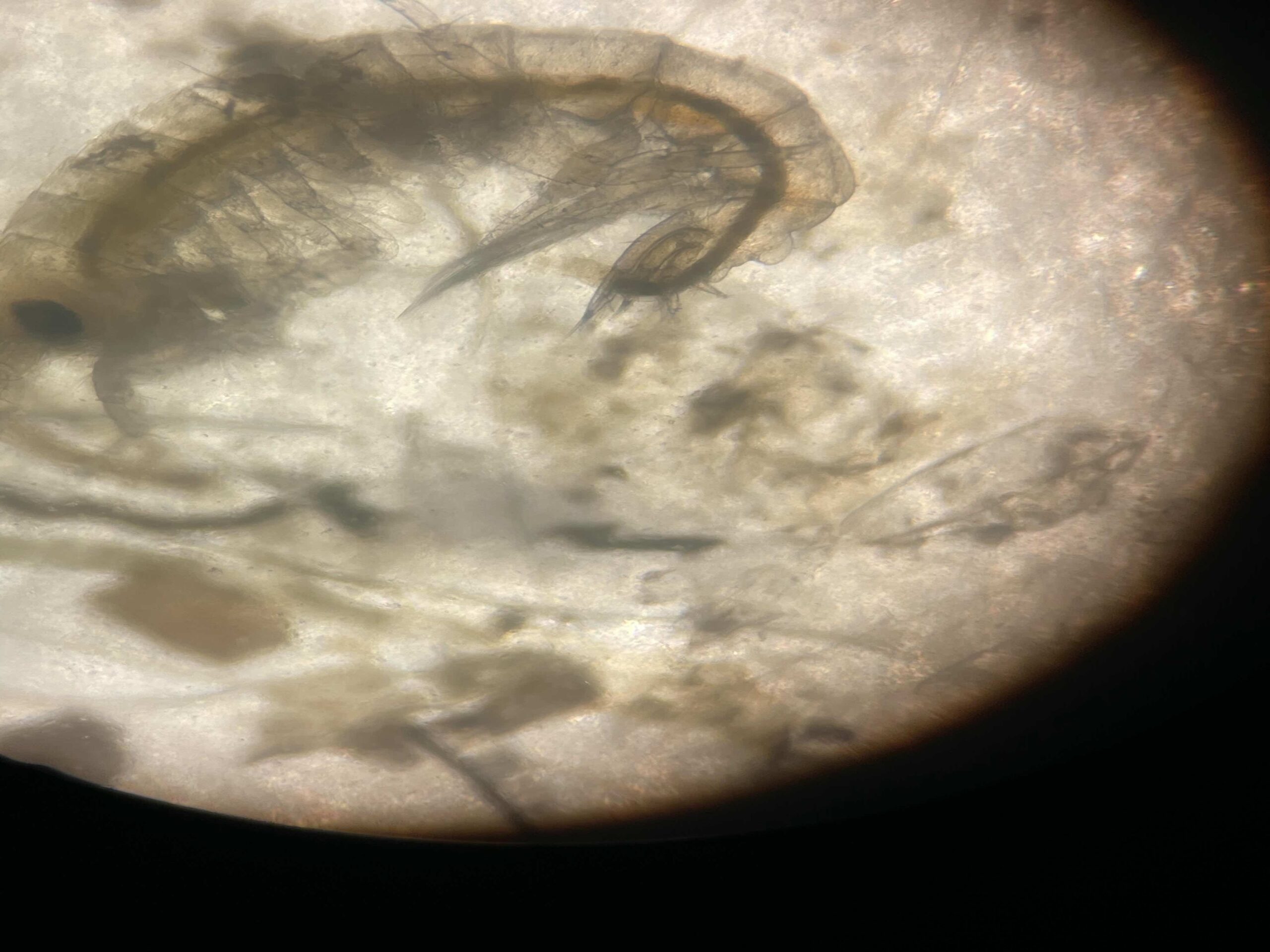
Along with this lack of whales, there does seem to be a lack of these “high calorie zoop species”. Our team has most frequently collected samples primarily comprising of Atylus tridens, a lower calorie prey type. In fact, during one of our earlier kayak training days this field season we collected 2,019 individual A. tridens. However, since this day we have collected sparse amounts of zooplankton in our samples, ranging from zero to 121 in a given sample. Our total zoop count thus far is 2,524 zooplankton, a third of the total zooplankton collected last field season.
Fig 3: Image of an Atylus tridens under a microscope.
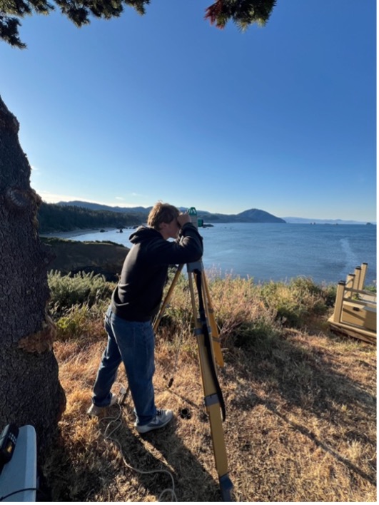
As for whale presence, we have been observing many whales blows near Hell’s Gate as mentioned in last week’s blog written by fellow intern Miranda Fowles. From our cliff site, it has been difficult to know whether these are gray whales or a different kind of whale, leading us to venture out to the Heads to get a better look. The persistence of whales in this area is certainly unusual, and perhaps it can be explained by a larger amount of higher calorie zooplankton species in the Hell’s Gate area.
Fig 4: Dawson tracking blows by Hell’s Gate with the theodolite.
Being part of the TOPAZ/JASPER project, I have become exposed to what the true meaning is behind “fieldwork,” including learning how to be flexible and adapt to new challenges every day. What I have most enjoyed is the team’s ability to overcome any new hurdle together as a unit. My dad often says, “You learn something new every day,” and this internship couldn’t embody this quote more. In just these 5 weeks, it almost feels like my head is now a couple sizes bigger.
Before this experience, I never thought much about how one might track a whale or how different microscopic species could have such a profound impact on a whale’s decision to forage. Now I feel I understand just how important these less than obvious factors are and the effort which goes behind understanding these relationships. I can only hope future opportunities teach me as much as joining the TOPAZ/JASPER legacy has—it’s an experience that, even just a few days into the 2025 field season, I knew would be hard to match.
Fig 4: Dawson (navigator) and Miranda (sampler) during kayak training on their way to Mill Rocks.
Hildebrand, L., Bernard, K. S., & Torres, L. G. (2021). Do Gray Whales Count Calories? Comparing Energetic Values of Gray Whale Prey Across Two Different Feeding Grounds in the Eastern North Pacific. Frontiers in Marine Science, 8, 683634. https://doi.org/10.3389/fmars.2021.683634
By Rachel Kaplan, PhD candidate, Oregon State University College of Earth, Ocean, and Atmospheric Sciences and Department of Fisheries, Wildlife, and Conservation Sciences, Geospatial Ecology of Marine Megafauna Lab
At the beginning of a graduate program, it’s common for people to tell you how quickly the time will pass, but hard to imagine that will really be the case. Suddenly, I’ve been working on my PhD for almost five years, and I’ll defend in just over two weeks. As I look back, I am amazed by how much I have learned and grown during this time, and how all the different parts of my graduate school experience have woven together. I began my program in 2020 with an intense “bootcamp” of oceanographic coursework, and am ending in 2025 with new analytical skills, a few publications, and a ton of new thoughts about whales and the zooplankton krill, the subjects of my research. My PhD work encapsulates all those different elements in an exploration of ecological relationships between baleen whale predators and their krill prey – which I now see as an expression of oceanographic and atmospheric processes.
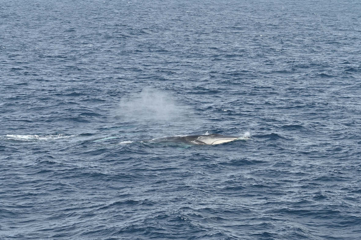
Figure 1. One of my favorite sightings during my PhD fieldwork was a group of seven fin whales in Antarctica, on Christmas 2024. Photo: Rachel Kaplan
Oceanographic processes drive prey quantity and quality across time and space, shaping the preyscape encountered by predators on their foraging grounds and driving habitat use (Fleming et al., 2016; Ryan et al., 2022). Aspects of prey including distribution, energy density, and biomass therefore represent mechanistic links between ocean and atmospheric conditions (e.g., El Niño Southern Oscillation cycles, circulation patterns, and upwelling processes) and diverse aspects of marine predator ecology, including spatiotemporal distributions, foraging behaviors, reproductive success, population size, and health. Both predator and prey species are impacted by environmental variability and climate change (e.g., Hauser et al., 2017; Atkinson et al., 2019; Perryman et al., 2021), and events like marine heatwaves and harmful algal blooms can force ecosystem changes on short, seasonal time scales (e.g. McCabe et al., 2016; Fisher et al., 2020). However, many marine species have some degree of plasticity that allows them to still accomplish life history events in the face of ecosystem variability (e.g., Lawrence, 1976; Oestreich, 2022), which may provide the capacity to adapt to climate change processes.
Observing and describing predator-prey relationships is complex due to the scale-dependent nature of these relationships (Levin, 1992). Each chapter of my dissertation considered krill, a globally-important prey type, from the perspective of baleen whales, which are krill predators. Chapter 2 used a comparative analysis to identify the optimal spatial scale at which to observe baleen whale-krill relationships on the Northern California Current (NCC) foraging grounds. We found correlations at a 5 km scale to be strongest, which can provide a useful starting point for further studies in the NCC and other systems. Chapter 3 used this spatial scale to compare several aspects of krill prey quality and quantity as predictors of humpback whale (Megaptera novaeangliae) distributions in the NCC. The best performing metric was a species, season, and spatially informed krill swarm biomass variable – yet the comparable performance of a simple acoustic abundance metric indicated that it can act as a reliable proxy for biomass. This finding may be advantageous for future research, as measuring the acoustic proxy is less computationally intensive and relies on fewer datastreams. Interestingly, one of this study’s best-performing models was based on only the proportion of Thysanoessa spinifera in krill swarms, which is also a highly accessible variable due to effective krill species distribution modeling in the NCC (Derville et al., 2024). Integrating the acoustic abundance proxy and krill species distribution predictions, two relatively simple metrics, could support predictions of humpback whale distributions in the NCC and inform whale-prey research in other ecosystems.
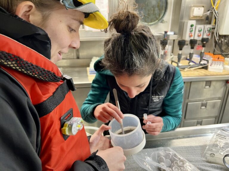
Figure 2. Collecting samples of individual krill gave us the opportunity to learn about their quality as prey for whales in the Northern California Current. Photo: Courtney Flatt
Studies relating predator foraging to prey characteristics often rely on metrics such as prey biomass or energy density (Schrimpf et al., 2012; Savoca et al., 2021; Cade et al., 2022), but the tendency of krill to form aggregations introduces dimensionality to krill prey quality. Chapter 4 showed that elements of krill swarm structure (particularly depth, proportion of T. spinifera, and metrics describing how krill occupy space within swarms) may be mechanistic drivers of variable blue, fin and humpback whale distribution patterns on the NCC foraging grounds. These findings suggest that krill swarm characteristics may be important links between baleen whales and the foraging environment. Swarm characteristics may be considered a component of krill prey quality for baleen whales, and future research could illuminate direct causal relationships between oceanographic conditions, krill swarming responses, and niche expression in baleen whale predators.
The relationships between baleen whale distributions and krill quantity and quality explored in the first chapters of my dissertation may also shed light on other aspects of baleen whale ecology. The final chapter considers overwintering trends in global baleen whale populations, and examines the wintertime Western Antarctic Peninsula (WAP) as a case study. Extended humpback whale presence on the WAP feeding grounds may be driven by the profitable feeding areas and elevated energy content of krill during the winter months, and may reflect the high energetic needs of certain demographic subgroups (e.g. lactating females, juveniles). Wintertime humpback whale presence may also reflect adaptation to multifaceted competitive pressure on krill resources that are declining due to climate change (Atkinson et al., 2019), including consumption by growing baleen whale populations (Johnston et al., 2011) and a fishery whose catch limits may be impacting krill predators (Watters et al., 2020; Savoca et al., 2024). This work demonstrates how investigating prey quality during the winter months can contextualize baleen whale overwintering on the foraging grounds. It also provides a meaningful violation of the canonical baleen whale migration paradigm central to marine mammal science, which may lessen the efficacy of whale monitoring programs and management policies.
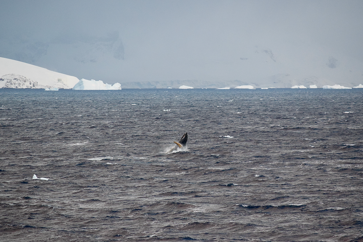
Figure 3. We were surprised to see humpback whales like this one in Antarctica during the winter months — which raised a number of questions about overwintering of baleen whales on foraging grounds around the world. Photo: Giulia Wood
Management efforts that aim to mitigate risk to whales often hinge on predictive modeling of whale distributions. Species distribution models (SDMs) can provide managers with spatially and temporally explicit predictions of protected species occurrences (Wikgren et al., 2014; Santora et al., 2020), but species distributions in rapidly changing ecosystems are difficult to predict (Muhling et al., 2020). Findings from this dissertation may inform modeling efforts by suggesting meaningful predictor variables for SDMs, such as krill species on the NCC foraging grounds and swarm energy density at the WAP. This work also speaks to meaningful spatial scales for analyzing predator-prey relationships (i.e., 5 km), and relevant elements of temporal variability (e.g., seasonal cycles of krill energy density).
Just as marine predator-prey relationships are shaped by ocean processes, they likewise have consequences for those processes. For example, krill and other zooplankton are capable of generating large-scale mixing that can overcome stratification of water masses and alter water column structure (Noss and Lorke, 2014). Baleen whales influence global carbon cycles due to the huge amount of prey they consume (Savoca et al., 2021; Pearson et al., 2023) and transport important nutrients along the “great whale conveyer belt” during their vast migrations (Roman et al., 2025). Baleen whales seek krill as an essential prey resource on foraging grounds around the globe, and the impact of this trophic interaction scales up, with implications for ecosystem functioning and management. Continued research into the spatiotemporally dynamic relationships between krill and baleen whales improves our understanding of ocean functioning, and can improve our capacity to live as part of this system.
References
Atkinson, A., Hill, S. L., Pakhomov, E. A., Siegel, V., Reiss, C. S., Loeb, V. J., Steinberg, D. K., et al. 2019. Krill (Euphausia superba) distribution contracts southward during rapid regional warming. Nature Climate Change, 9: 142–147.
Cade, D. E., Kahane-Rapport, S. R., Wallis, B., Goldbogen, J. A., and Friedlaender, A. S. 2022. Evidence for Size-Selective Predation by Antarctic Humpback Whales. Frontiers in Marine Science, 9: 747788.
Derville, S., Fisher, J. L., Kaplan, R. L., Bernard, K. S., Phillips, E. M., and Torres, L. G. 2024. A predictive krill distribution model for Euphausia pacifica and Thysanoessa spinifera using scaled acoustic backscatter in the Northern California Current. Progress in Oceanography: 103388.
Fisher, J. L., Menkel, J., Copeman, L., Shaw, C. T., Feinberg, L. R., and Peterson, W. T. 2020. Comparison of condition metrics and lipid content between Euphausia pacifica and Thysanoessa spinifera in the northern California Current, USA. Progress in Oceanography, 188.
Fleming, A. H., Clark, C. T., Calambokidis, J., and Barlow, J. 2016. Humpback whale diets respond to variance in ocean climate and ecosystem conditions in the California Current. Glob Chang Biol, 22: 1214–24.
Hauser, D. D. W., Laidre, K. L., Stafford, K. M., Stern, H. L., Suydam, R. S., and Richard, P. R. 2017. Decadal shifts in autumn migration timing by Pacific Arctic beluga whales are related to delayed annual sea ice formation. Global Change Biology, 23: 2206–2217.
Johnston, S. J., Zerbini, A. N., and Butterworth, D. S. 2011. A Bayesian approach to assess the status of Southern Hemipshere humpback whales (Megaptera novaeangliae) with an application to Breeding Stock G. J. Cetacean Res. Manage.: 309–317. International Whaling Commission.
Lawrence, J. M. 1976. Patterns of Lipid Storage in Post-Metamorphic Marine Invertebrates. American Zoologist, 16: 747–762. Oxford University Press (OUP).
Levin, S. A. 1992. The Problem of Pattern and Scale in Ecology: The Robert H. MacArthur Award Lecture. Ecology, 73: 1943–1967.
McCabe, R. M., Hickey, B. M., Kudela, R. M., Lefebvre, K. A., Adams, N. G., Bill, B. D., Gulland, F. M., et al. 2016. An unprecedented coastwide toxic algal bloom linked to anomalous ocean conditions. Geophys Res Lett, 43: 10366–10376.
Muhling, B. A., Brodie, S., Smith, J. A., Tommasi, D., Gaitan, C. F., Hazen, E. L., Jacox, M. G., et al. 2020. Predictability of Species Distributions Deteriorates Under Novel Environmental Conditions in the California Current System. Frontiers in Marine Science, 7.
Noss, C., and Lorke, A. 2014. Direct observation of biomixing by vertically migrating zooplankton. Limnology and Oceanography, 59: 724–732. Wiley.
Oestreich, W. 2022. Acoustic signature reveals blue whales tune life‐history transitions to oceanographic conditions. Functional Ecology. https://besjournals.onlinelibrary.wiley.com/doi/10.1111/1365-2435.14013 (Accessed 20 September 2024).
Pearson, H. C., Savoca, M. S., Costa, D. P., Lomas, M. W., Molina, R., Pershing, A. J., Smith, C. R., et al. 2023. Whales in the carbon cycle: can recovery remove carbon dioxide? Trends in Ecology & Evolution, 38: 238–249.
Perryman, W. L., Joyce, T., Weller, D. W., and Durban, J. W. 2021. Environmental factors influencing eastern North Pacific gray whale calf production 1994–2016. Marine Mammal Science, 37: 448–462. Wiley.
Roman, J., Abraham, A. J., Kiszka, J. J., Costa, D. P., Doughty, C. E., Friedlaender, A., Hückstädt, L. A., et al. 2025. Migrating baleen whales transport high-latitude nutrients to tropical and subtropical ecosystems. Nature Communications, 16: 2125. Nature Publishing Group.
Ryan, J. P., Benoit-Bird, K. J., Oestreich, W. K., Leary, P., Smith, K. B., Waluk, C. M., Cade, D. E., et al. 2022. Oceanic giants dance to atmospheric rhythms: Ephemeral wind-driven resource tracking by blue whales. Ecology Letters, 25: 2435–2447.
Santora, J. A., Mantua, N. J., Schroeder, I. D., Field, J. C., Hazen, E. L., Bograd, S. J., Sydeman, W. J., et al. 2020. Habitat compression and ecosystem shifts as potential links between marine heatwave and record whale entanglements. Nat Commun, 11: 536.
Savoca, M. S., Czapanskiy, M. F., Kahane-Rapport, S. R., Gough, W. T., Fahlbusch, J. A., Bierlich, K. C., Segre, P. S., et al. 2021. Baleen whale prey consumption based on high-resolution foraging measurements. Nature, 599: 85–90.
Savoca, M. S., Kumar, M., Sylvester, Z., Czapanskiy, M. F., Meyer, B., Goldbogen, J. A., and Brooks, C. M. 2024. Whale recovery and the emerging human-wildlife conflict over Antarctic krill. Nature Communications, 15: 7708. Nature Publishing Group.
Schrimpf, M., Parrish, J., and Pearson, S. 2012. Trade-offs in prey quality and quantity revealed through the behavioral compensation of breeding seabirds. Marine Ecology Progress Series, 460: 247–259.
Watters, G. M., Hinke, J. T., and Reiss, C. S. 2020. Long-term observations from Antarctica demonstrate that mismatched scales of fisheries management and predator-prey interaction lead to erroneous conclusions about precaution. Scientific Reports, 10: 2314.
Wikgren, B., Kite-Powell, H., and Kraus, S. 2014. Modeling the distribution of the North Atlantic right whale Eubalaena glacialis off coastal Maine by areal co-kriging. Endangered Species Research, 24: 21–31.
Dr. Enrico Pirotta (CREEM, University of St Andrews) and Dr. Leigh Torres (GEMM Lab, MMI, OSU)
The health of animals affects their ability to survive and reproduce, which, in turn, drives the dynamics of populations, including whether their abundance trends up or down. Thus, understanding the links between health and reproduction can help us evaluate the impact of human activities and climate change on wildlife, and effectively guide our management and conservation efforts. In long-lived species, such as whales, once a decline in population abundance is detected, it can be too late to reverse the trend, so early warning signals are needed to indicate how these populations are faring.
We worked on this complex issue in a study that was recently published in the Journal of Animal Ecology. In this paper, we developed a new statistical approach to link three key components of the health of a Pacific Coast Feeding Group (PCFG) gray whale (namely, its body size, body condition, and stress levels) to a female’s ability to give birth to a calf. We were able to inform these metrics of whale health using an eight-year dataset derived from the GRANITE project of aerial images from drones for measurements of body size and condition, and fecal samples for glucocorticoid hormone analysis as an indicator of stress. We combined these data with observations of females with or without calves throughout the PCFG range over our study period.
We found that for a female to successfully have a calf, she needs to be both large and fat, as these factors indicate if the female has enough energy stored to support reproduction that year (Fig. 1). Remarkably, we also found indication that females with particularly high stress hormone levels may not get pregnant in the first place, which is the first demonstration of a link between stress physiology and vital rates in a baleen whale, to our knowledge.
Figure 1. Taken from Pirotta et al. (2025), Fig. 5. Combined relationship of PCFG gray whale length and nutritional state (combination of body size and condition) in the previous year with calving probability, colored by whether the model estimated an individual to have calved or not at a given reproductive opportunity.
Our study’s findings are concerning given our previous research indicating that gray whales in this PCFG sub-group have been growing to shorter lengths over the last couple of decades (Pirotta et al. 2023), are thinner than animals in the broader Eastern North Pacific gray whale population (Torres et al, 2022), and show an increase in stress-related hormones when exposed to human activities (Lemos et al, 2022; Pirotta et al. 2023). Furthermore, in our recent study we also documented that there are fewer young individuals than expected for a growing or stable population (Fig. 2), which can be an indicator of a population in decline since there may not be many individuals entering the reproductive adult age groups. Altogether, our results act as early warning signals that the PCFG may be facing a possible population decline currently or in the near future.
Figure 2. Taken from Pirotta et al. (2025), Fig. 1. Age structure diagram for 139 PCFG gray whales in our dataset. Each bar represents the number of individuals of a given age in 2023, with the color indicating the proportion of individuals of that age for which age is known (vs. estimated from a minimum estimate following Pirotta, Bierlich, et al., 2024). The red line reports a smooth kernel density estimate of the distribution.
These findings are sobering news for Oregon residents and tourists who enjoy watching these whales along our coast every summer and fall. We have gotten to know many of these whales so well – like Scarlett, Equal, Clouds, Lunita, and Pacman, who you can meet on our IndividuWhale website – that we wonder how they will adapt and survive as their once reliable habitat and prey-base changes. We hope our work sparks collective and multifaceted efforts to reduce impacts on these unique PCFG whales, and that we can continue the GRANITE project for many more years to come to monitor these whales and learn from their response to change.
This work exemplifies the incredible value of long-term studies, interdisciplinary methods, and effective collaboration. Through many years of research on this gray whale group, we have collected detailed data on diverse aspects of their behavior, ecology and life history that are critical to understanding their response to disturbance and environmental change, which are both escalating in the study region. We are incredibly grateful to the following members of the PCFG Consortium for contributing sightings and calf observation data that supported this study: Jeff Jacobsen, Carrie Newell, NOAA Fisheries (Peter Mahoney and Jeff Harris), Cascadia Research Collective (Alie Perez), Department of Fisheries and Oceans, Canada (Thomas Doniol-Valcroze and Erin Foster), Mark Sawyer and Ashley Hoyland, Wendy Szaniszlo, Brian Gisborne, Era Horton.
Did you enjoy this blog? Want to learn more about marine life, research, and conservation? Subscribe to our blog and get a weekly alert when we make a new post! Just add your name into the subscribe box below!
References:
Lemos, Leila S., Joseph H. Haxel, Amy Olsen, Jonathan D. Burnett, Angela Smith, Todd E. Chandler, Sharon L. Nieukirk, Shawn E. Larson, Kathleen E. Hunt, and Leigh G. Torres. “Effects of Vessel Traffic and Ocean Noise on Gray Whale Stress Hormones.” Scientific Reports 12, no. 1 (2022): 18580. https://dx.doi.org/10.1038/s41598-022-14510-5.
Pirotta, Enrico, Alejandro Fernandez Ajó, K. C. Bierlich, Clara N Bird, C Loren Buck, Samara M Haver, Joseph H Haxel, Lisa Hildebrand, Kathleen E Hunt, Leila S Lemos, Leslie New, and Leigh G Torres. “Assessing Variation in Faecal Glucocorticoid Concentrations in Gray Whales Exposed to Anthropogenic Stressors.” Conservation Physiology 11, no. 1 (2023). https://dx.doi.org/10.1093/conphys/coad082.
Torres, Leigh G., Clara N. Bird, Fabian Rodríguez-González, Fredrik Christiansen, Lars Bejder, Leila Lemos, Jorge Urban R, et al. “Range-Wide Comparison of Gray Whale Body Condition Reveals Contrasting Sub-Population Health Characteristics and Vulnerability to Environmental Change.” Frontiers in Marine Science 9 (2022). https://doi.org/10.3389/fmars.2022.867258. https://www.frontiersin.org/article/10.3389/fmars.2022.867258
Baleen whales must navigate a seemingly featureless world to locate the resources they need to survive. The task of finding prey to feed on in the vast seascapes relies on the use of several sensory modalities that operate at different scales (Torres 2017; Figure 1). For example, baleen whale vision is believed to be rather limited, with the ability to see objects about 10-100 meters away. Yet, baleen whale somatosensory perception of oceanographic stimuli is thought to be on the order of 100-1000s kilometers. This diversity in sensory ability has led scientists to believe that whales, in fact all animals, perceive cues and make decisions at several scales. As ecologists, we endeavor to understand why and when animals are found (or not found) in certain locations as this knowledge allows us to better manage and conserve animal populations. With this information we can aim to minimize potential anthropogenic disturbance and protect important resource areas, such as foraging or nursing grounds. In order to accomplish this goal, we ourselves must conduct studies and test hypotheses at several scales (Levin 1992; Hobbs 2003). As someone who tackles spatial foraging ecology questions, I am particularly interested in understanding whale behavior and movement in the context of feeding. Since accurately measuring predator and prey distribution at the same scales can be challenging, we often resort to environmental variables to serve as proxies for prey, whereby we look for correlations between environmental variables and whales to understand and predict the distribution of our population.
Figure 1. Schematic of hypothetical interchange of sensory modalities used by baleen whales to locate prey at variable scales. X-axis represents log distance to prey from micro (left) to macro (right). Y-axis represents the relative use of each sensory modality between 0 (no contribution) to 10 (highest contribution). Each line and color represent a different sensory modality. Figure taken and caption adapted from Torres 2017.
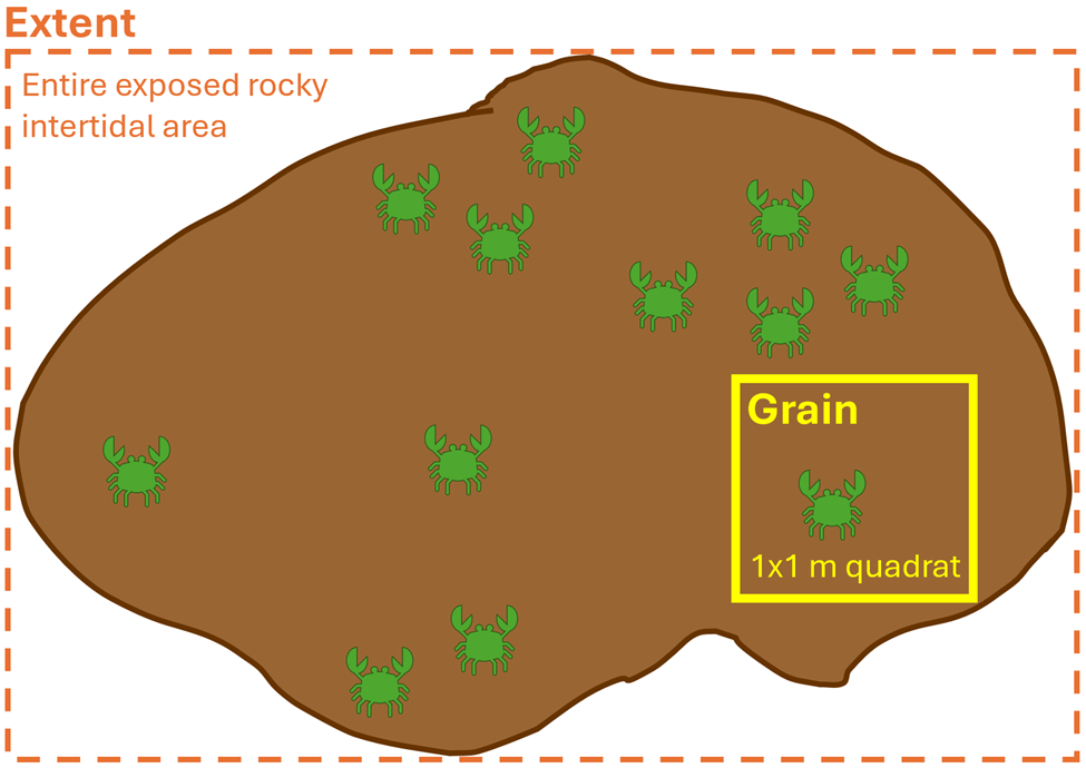
What do I mean when I use the word ‘scale’? The term scale is typically explained by two components: grain and extent (Wiens 1989). The grain is the finest resolution measured; in other words, how detailed we are measuring. The extent is the overall coverage of what we are measuring. These components can be applied to both spatial scale and temporal scale. For example, spatially, if we were using a 1×1 meter sampling quadrat to count the number of crabs on a rocky shore, then our grain would be the 1 m2 quadrat and the extent would be the entire exposed rocky intertidal area that we are surveying (Figure 2). Temporally, if we placed a temperature logger at the mouth of Yaquina Bay that took a temperature recording every minute for two years, then our grain would be one minute and the extent would be two years. So, when designing a study, it is imperative for us to decide on the spatiotemporal scales of the ecological questions we are asking and the hypotheses we are testing, as it will inform what data we need to collect. When making this decision, it is important to think about the scale at which the ecological process happens, as opposed to the scale at which we can observe the process (Levin 1992). In other words, we need to think from the perspective of our study species, as opposed to from our own human perspective. Making informed and ecologically reasonable decisions regarding the choice of scale relies on having prior knowledge of an animal’s biology, such as knowing that baleen whales might see a prey patch that is 50 meters away, but it may also somatosensorily perceive an oceanic front where zooplankton prey aggregate from 500 kilometers away.
Figure 2. Schematic of spatial scale where the extent (depicted by dashed orange box) is the entire exposed rocky intertidal area being surveyed and the grain (solid yellow box) is the 1×1 m quadrat being used to count crabs.
There is a wealth of studies that have explored space use patterns of wildlife relative to environmental variables to better understand foraging behavior. I want to share a couple from the marine mammal realm with you that I find particularly fascinating. In their 2018 study, González García and colleagues used opportunistic sightings of blue whales around the Azorean islands of Portugal and modeled their distribution patterns relative to physiographic and oceanographic variables summarized at different spatial (fine [1-10 km] and meso [10-100 km]) and temporal (daily, weekly, monthly) scales. The two variables that were most correlated with blue whale occurrence was distance from the coast and eddy kinetic energy (a measure of mesoscale variability of ocean dynamics). Both of these variables were interestingly found to be scale invariant, meaning that no matter which spatial and temporal scale was investigated, the relationship between blue whales and these two variables stayed the same; blue whale occurrence increased with increasing distance from the coast and was maximal at an eddy kinetic energy value of 0.007 cm2/s2 (Figure 3).
Figure 3. Functional response curves between presence of Azorean blue whales and distance to the coast (panel 1 on left) and eddy kinetic energy (panel 2 on right). The top row of each panel represents the low spatial scale and the bottom row represents the high spatial scale. Each column represents a different temporal scale (from left to right: daily, weekly, monthly). Note that the general shape of the relationship remains similar across all spatiotemporal scales and that the peak of the curves tend to occur at the same values for distance to coast and eddy kinetic energy across all scales. Figures taken from González García et al. 2018.
However, not all studies find scale invariant relationships. For example, Cotté and co-authors (2009) found that habitat use of Mediterranean fin whales was very much scale dependent. At a large scale (700-1,000 km and annual), fin whales were more densely aggregated during the summer in the Western Mediterranean where there was consistently colder water than in the winter. However, at a meso scale (20-100 km and weekly-monthly), fin whale densities were highest in areas where there were steep changes in temperature, as opposed to consistently cold temperatures. The authors explain that these differences in fin whale density and temperature at different scales are likely due to whale movement being driven by annually persistent prey abundance at the large scale, but at the meso scale, where prey aggregations are less predictable, the fin whales’ distribution becomes more driven by areas of physical ocean mixing.
As I investigate the environmental drivers of individual gray whale space use using our 8-year GRANITE (Gray whale Response to Ambient Noise Informed by Technology and Ecology) dataset, these studies (and many more) are at the top of my mind to interpret the patterns we are detecting. Our goal is to quantify and describe what environmental conditions (1) lead to a higher probability of a gray whale being seen in our central Oregon coast study area (~70 km) at a daily scale, and (2) influence space use patterns (activity range, residency, activity center) of different individual whales at annual scales. Our results show both consistency and variation in the environmental drivers of gray whales across these scales, leading me to deeply consider how gray whales make decisions at different points in their lives, based on information gained through various senses, to maximize their chances of capturing food. Previous work from the GEMM Lab on the relationships between gray whales and prey, at both fine (read more here) and large (read more here) scales have guided my work by providing specific hypotheses regarding environmental variables and lag times for me to test. Investigating the environmental drivers of animal space use and behavior is exciting work as it reveals that no single environmental variable determines animal distribution, but rather that multiple processes are happening concomitantly that animals respond to at different scales continually. It is only by studying animal space use patterns across spatiotemporal scales that we can begin to understand their complex decision-making patterns.
Did you enjoy this blog? Want to learn more about marine life, research, and conservation? Subscribe to our blog below and get a monthly message when we post a new blog. Just add your name and email into the subscribe box below.
References
Cotté, C., Guinet, C., Taupier-Letage, I., Mate, B., & Petiau, E. (2009). Scale-dependent habitat use by a large free-ranging predator, the Mediterranean fin whale. Deep Sea Research Part I: Oceanographic Research Papers, 56(5), 801-811.
González García, L., Pierce, G. J., Autret, E., & Torres-Palenzuela, J. M. (2018). Multi-scale habitat preference analyses for Azorean blue whales. PLoS One, 13(9), e0201786.
Hobbs, N. T. (2003). Challenges and opportunities in integrating ecological knowledge across scales. Forest Ecology and Management, 181(1-2), 223-238.
Levin, S. A. (1992). The problem of pattern and scale in ecology: the Robert H. MacArthur award lecture. Ecology, 73(6), 1943-1967.
Torres, L. G. (2017). A sense of scale: Foraging cetaceans’ use of scale‐dependent multimodal sensory systems. Marine Mammal Science, 33(4), 1170-1193.
Wiens, J. A. (1989). Spatial scaling in ecology. Functional ecology, 3(4), 385-397.
By Natalie Nickells, visiting PhD Student, British Antarctic Survey
For the last three months, I’ve been lucky enough to be welcomed into the GEMM lab as a visiting PhD student to work on the acoustic data from hydrophones in CATS tags deployed on gray whales. This work has been a huge change for me! I’ve gone from studying Antarctic baleen whale foraging, the topic of my PhD, from a distance at my desk in Cambridge England, to studying PCFG gray whales in Newport- and finally being in the same country, state, and even county to the whales I am studying! Unlike my Antarctic research, where whale blows in the distance become tiny points in a sea of data, listening to the CATS tag data has allowed me to really connect with these animals on an emotional level, as I’ve spent days, weeks and months listening to the world as they hear it.
Humans are fundamentally visual creatures- we take in information through sight first, with hearing probably our second, or for some even third, sense in line. However, for marine mammals, the same cannot be said: their world is auditory first. This fact is an important realisation to get our heads around, highlighted beautifully by the phrase “the ears are the window to the soul of the whale” (Sonic Sea (2017)) or Tim Donaghy’s emotive statement that “a deaf whale is a dead whale”. High levels of ocean noise therefore have a huge impact on baleen whales. Imagine trying to do your groceries or find a friend while blindfolded or in a thick fog– you might struggle to access food or communicate with others, and your stress would certainly be high. To succeed, you would likely need to change your behaviour.
Behavioural changes in response to ocean noise are observed in baleen whales: for example, humpback whales change their foraging behaviour when ship noise increases (Blair et al., 2016), and gray whales have been shown to call more frequently and possibly more loudly in conditions of high ocean noise (Dahlheim & Castellote, 2016). However, even in the absence of notable behaviour change due to ocean noise, North Atlantic right whales may still be experiencing a stress response. When shipping traffic in the Bay of Fundy significantly decreased in the aftermath of 9/11, North Atlantic right whales in the area had decreased chronic stress levels (Rolland et al., 2012).
Previous work by the GEMM lab observed this stress response to ocean noise in gray whales. They found a correlation between high levels of glucocorticoid (a stress indicator) in male gray whale faeces with high vessel noise and vessel counts in the area. Vessel noise was measured using two static hydrophones off the Oregon coast, and it was assumed all animals in the area experienced the same noise (Lemos et al., 2022; Pirotta et al., 2023). However, a static hydrophone is an imperfect measure of the sound levels a mobile animal experiences, particularly as we might expect animals to change behaviour when disturbed (Sullivan & Torres, 2018). This previous work became the starting point for the question I have addressed during my time in the GEMM Lab: can we measure and characterise the sound levels an individual whale was exposed to? Enter CATS tags. These are suction-cup tags fitted with a host of sensors, which have been used by the GEMM lab since 2021 (see Image 1). So far, they have mostly been used for their accelerometry data (Colson et al. (in press), see also Kate’s blog post). However, the GEMM lab had the foresight to put hydrophones on these tags, and as a result I was welcomed into the lab by a bumper-crop of hydrophone data just waiting to be analysed!
Image 1: A gray whale (“Slush”) being tagged with a CATS tag and Natalie (right) with the same tag.
This tag data is particularly valuable, not only for its ability to follow the acoustic world of an individual whale, but also due to the whole suite of data that comes with the acoustics: essentially, the acoustic data comes with behavioural data. Or at least, it comes with data from which we can infer behaviour (Colson et al, in press)! Incorporating behaviour into passive acoustics work hugely strengthens its ecological usefulness (Oestreich et al., 2024). We can hear what an individual whale is hearing, and we can also infer what they were doing before, during, and after they heard or made that sound. Having behavioural data also means that we can ground-truth the sounds we hear. When hearing an interesting sound, I can go back to the video data and accelerometer data to check what the whale sees, what its body-position is doing (e.g., is it headstand foraging?) and the speed and direction of its travel. Context is key!
The importance of context was highlighted in my very first week here in the GEMM lab. I became very interested in a sound I could hear frequently when the whale would surface- a distorted bark-like noise, but the whale was surely too far offshore for any barking dog to be heard? And almost every time the whale surfaced? After a few days pondering, I shared my mystery with Leigh, who laughingly revealed that one of the whale-watching boats in this area has a ‘whale-alerting’ dog on board! Sometimes if it sounds like a dog… it’s a dog! Besides my slightly anticlimactic discovery of dogs barking, committing time to listening to the tags and hearing what the whales hear, has been a magical experience. My favourite hydrophone sound, that still gets me excited when I hear it, is the gray whale ‘bongo call’- or as it’s more formally known in the literature, M1 vocalisation (Guazzo et al., 2019). I’ll let you decide which name is more appropriate! I first heard this call when investigating a time on “Scarlett’s” tag when we knew her 14 year-old daughter “Pacman” had been close: about 15 minutes before “Pacman” appears on the video, Scarlett makes this call (you can play the clip below to listen). In “Lunita’s” tag, we even hear this call three times in a row!
Image 2: A ‘bongo call’ made by “Scarlett” when her daughter “Pacman” was nearby.
Relatively little research has been done on gray whale calls compared to other more studied species like humpbacks. Most of this research has taken place on gray whale migratory routes (Guazzo et al., 2019, 2017; Burnham et al. 2018) or in captivity (Fish et. al, 1974 ) so these tag recordings could be a valuable addition to a small sample from the foraging grounds (Clayton et al., 2023; Haver et al., 2023)- as well as being very personally exciting to hear!
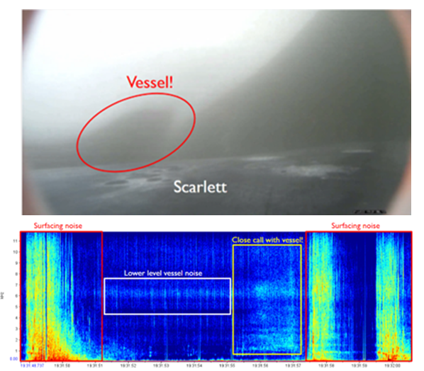
We’ve also been able to use the tag hydrophone data to look at close calls with ships. As I was going through the data on “Scarlett’s” tag, I noticed a spike in vessel noise. Looking at the video from the same timestamp, I could see a small vessel passing directly over her as she surfaced. At the time this vessel passed over her, the tag was only 0.8 m under the surface of the water!
Image 3: A close encounter between a small vessel and “Scarlett”, shown both on the video from the CATS tag (top) and the spectrogram (bottom). The close call is outlined in a yellow box, when a greater intensity of noise occurred as illustrated by the brighter colour intensity compared to the white box (quieter vessel noise). Brighter colours denote a louder volume. The red boxes show surfacing noise- this can essentially be ignored when interpreting the echogram for our purposes.
Sometimes vessels may be more distant, but possibly equally harmful: we have seen vessel noise from larger and presumably more distant vessels dominate the soundscape in some of the tag data. Remembering that to a whale, the sonic world is as important as the visual world is to us, this elevated background noise from ships could have major consequences. So, the first step is to try to quantify the gray whales’ exposure to this vessel noise. I’ve been running some systematic sampling on the tag data to try to quantify background noise levels, and how this changes depending on the time of day: do individual whales experience the same daily spikes in ocean noise that were detected on the static hydrophones, at around 6am and noon due to vessel traffic (Haver et al., 2023)? If not, are they taking evasive action to avoid these spikes? These are just some of the questions that these CATS tags can help us answer, although ideally we need longer acoustic data recordings to capture day and night data, as well as potentially improving the hydrophones on the CATS tags themselves to minimise the impacts of tag interference and random noise.
When explaining to the public what it is to be a PhD student, I often refer to myself as a ‘scientist in training’, or to young children, a ‘baby scientist’. As I look toward my departure from the GEMM lab, I hope to have developed into at least a scientific toddler, having gained the ability to walk through reams of acoustic data with (relative) independence. More than that, I’m excited to take home a refreshed sense of curiosity about what drives marine mammals to behave as they do, an openness to collaboration and new approaches, and a large dose of ‘American emotion’! Let’s hope my British colleagues can handle it!
My heartfelt thanks to all those who welcomed me so warmly at the GEMM lab and Oregon State University, particularly my mentors Leigh Torres and Samara Haver.
Did you enjoy this blog? Want to learn more about marine life, research, and conservation? Subscribe to our blog and get a weekly alert when we make a new post! Just add your name into the subscribe box below!
Bibliography
Sonic Sea (2017) Directed by Michelle Dougherty [Film] Distributed by the Natural Resources Defense Council.
Burnham, R., Duffus, D. & Mouy, X. (2018) Gray Whale (Eschrictius robustus) Call Types Recorded During Migration off the West Coast of Vancouver Island. Frontiers in Marine Science. 5, 329. doi:10.3389/fmars.2018.00329.
Colson, K., E. Pirotta L. New, D Cade, J Calambokidis, K. Bierlich, C Bird, A Fernandez Ajó, L. Hildebrand, A. Trites, L. Torres. (in press). Using accelerometry tags to quantify gray whale foraging behavior. Marine Mammal Science.
Clayton, H., Cade, D.E., Burnham, R., Calambokidis, J. & Goldbogen, J. (2023) Acoustic behavior of gray whales tagged with biologging devices on foraging grounds. Frontiers in Marine Science. 10, 1111666. doi:10.3389/fmars.2023.1111666.
Dahlheim, M. & Castellote, M. (2016) Changes in the acoustic behavior of gray whales Eschrichtius robustus in response to noise. Endangered Species Research. 31, 227–242. doi:10.3354/esr00759.
Fish, J.F., Sumich, J.L. & Lingle, G.L. (n.d.) Sounds Produced by the Gray Whale, Eschrichtius robustus.
Guazzo, R., Schulman-Janiger, A., Smith, M., Barlow, J., D’Spain, G., Rimington, D. & Hildebrand, J. (2019) Gray whale migration patterns through the Southern California Bight from multi-year visual and acoustic monitoring. Marine Ecology Progress Series. 625, 181–203. doi:10.3354/meps12989.
Guazzo, R.A., Helble, T.A., D’Spain, G.L., Weller, D.W., Wiggins, S.M. & Hildebrand, J.A. (2017) Migratory behavior of eastern North Pacific gray whales tracked using a hydrophone array S. Li (ed.). PLOS ONE. 12 (10), e0185585. doi:10.1371/journal.pone.0185585.
Haver, S.M., Haxel, J., Dziak, R.P., Roche, L., Matsumoto, H., Hvidsten, C. & Torres, L.G. (2023) The variable influence of anthropogenic noise on summer season coastal underwater soundscapes near a port and marine reserve. Marine Pollution Bulletin. 194, 115406. doi:10.1016/j.marpolbul.2023.115406.
Lemos, L.S., Haxel, J.H., Olsen, A., Burnett, J.D., Smith, A., Chandler, T.E., Nieukirk, S.L., Larson, S.E., Hunt, K.E. & Torres, L.G. (2022) Effects of vessel traffic and ocean noise on gray whale stress hormones. Scientific Reports. 12 (1), 18580. doi:10.1038/s41598-022-14510-5.
Oestreich, W.K., Oliver, R.Y., Chapman, M.S., Go, M.C. & McKenna, M.F. (2024) Listening to animal behavior to understand changing ecosystems. Trends in Ecology & Evolution. S0169534724001459. doi:10.1016/j.tree.2024.06.007.
Pirotta, E., Fernandez Ajó, A., Bierlich, K.C., Bird, C.N., Buck, C.L., Haver, S.M., Haxel, J.H., Hildebrand, L., Hunt, K.E., Lemos, L.S., New, L. & Torres, L.G. (2023) Assessing variation in faecal glucocorticoid concentrations in gray whales exposed to anthropogenic stressors S. Cooke (ed.). Conservation Physiology. 11 (1), coad082. doi:10.1093/conphys/coad082.
Rolland, R.M., Parks, S.E., Hunt, K.E., Castellote, M., Corkeron, P.J., Nowacek, D.P., Wasser, S.K. & Kraus, S.D. (2012) Evidence that ship noise increases stress in right whales. Proceedings of the Royal Society B: Biological Sciences. 279 (1737), 2363–2368. doi:10.1098/rspb.2011.2429.
Sullivan, F.A. & Torres, L.G. (2018) Assessment of vessel disturbance to gray whales to inform sustainable ecotourism. The Journal of Wildlife Management. 82 (5), 896–905. doi:10.1002/jwmg.21462.
Celest Sorrentino, incoming master’s student, OSU Dept of Fisheries, Wildlife, and Conservation Sciences, GEMM Lab
It’s late June, a week before I head back to the West Coast, and I’m working one of my last shifts as a server in New York. Summer had just turned on and the humidity was just getting started, but the sun brought about a liveliness in the air that was contagious. Our regulars traded the city heat for beaches in the Hamptons, so I stood by the door, watching the flow of hundreds upon hundreds of people fill the streets of Manhattan. My manager and I always chatted to pass the time between rushes, and he began to ask me how I felt to move across the country and start my master’s program so soon.
“I am so excited!” I beamed, “Also a bit nervous–”
“Nervous? Why?
“Are you nervous you’ll become the person you’re meant to be?”
As a first-generation Hispanic student, I found solace in working in hospitality. Working in a restaurant for four years was a means to support myself to attain an undergraduate degree–but I’d be lying if I said I didn’t also love it. I found joy in orchestrating a unique experience for strangers, who themselves brought their own stories to share, each day bestowing opportunity for new friendships or new lessons. This industry requires you to be quick on your feet (never mess with a hungry person’s cacio e pepe), exuding a sense of finesse, continuously alert to your client’s needs and desires all the while always exhibiting a specific ambiance.
So why leave to start my master’s degree?
Fig 1: Me as a server with one of my regulars before his trip to Italy. You can never go wrong with Italian!
For anyone I have not had the pleasure yet to meet, my name is Celest Sorrentino, an incoming master’s student in the GEMM Lab this fall. I am currently writing to you from the Port Orford Field Station, located along the charming south coast of Oregon. Although I am new to the South Coast, my relationship with the GEMM Lab is not, but rather has been warmly cultivated ever since the day I first stepped onto the third floor of the Gladys Valley Building, as an NSF REU intern just two summers ago. Since that particular summer, I have gravitated back to the GEMM Lab every summer since: last summer as a research technician and this summer as a co-lead for the TOPAZ/JASPER Project, a program I will continue to spearhead the next two summers. (The GEMM Lab and me, we just have something– what can I say?)
In the risk of cementing “cornball” to my identity, pursuing a life in whale research had always been my dream ever since I was a little girl. As I grew older, I found an inclination toward education, in particular a specific joy that could only be found when teaching others, whether that meant teaching the difference between “bottom-up” and “top-bottom” trophic cascades to my peers in college, teaching my 11 year old sister how to do fun braids for middle school, or teaching a room full of researchers how I used SLEAP A.I. to track gray whale mother-calf pairs in drone footage.
Onboarding to the TOPAZ/JASPER project was a new world to me, which required me to quickly learn the ins and outs of a program, and eventually being handed the reins of responsibility of the team, all within 1 month and a half. While the TOPAZ/JASPER 2024 team (aka Team Protein!) and I approach our 5th week of field season, to say we have learned “so much” is an understatement.
Our morning data collection commences at 6:30 AM, with each of us alternating daily between the cliff team and kayak team.
For kayak team, its imperative to assemble all supplies swiftly given that we’re in a race against time, to outrun the inevitable windy/foggy weather conditions. However, diligence is required; if you forget your paddles back at lab or if you run out of charged batteries, that’s less time on the water to collect data and more time for the weather to gain in on you. We speed up against the weather, but also slow down for the details.
Fig 2: Throwback to our first kayak training day with Oceana (left), Sophia(middle), and Eden (right).
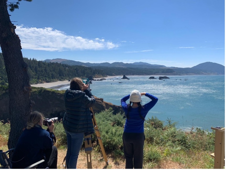
For cliff team, we have joined teams with time. At some point within the last few weeks, each of us on the cliff have had to uncover the dexterity within to become true marine mammal observers (for five or six hours straight). Here we survey for any slight shift in a sea of blue that could indicate the presence of a whale– and once we do… its go time. Once a whale blows, miles offshore, the individual manning the theodolite has just a few seconds to find and focus the reticle before the blow dissipates into the wind. If they miss it… its one less coordinate of that whale’s track. We speed up against the whale’s blow, but also slow down for the details.
Fig 3: Cliff team tracking a whale out by Mill Rocks!
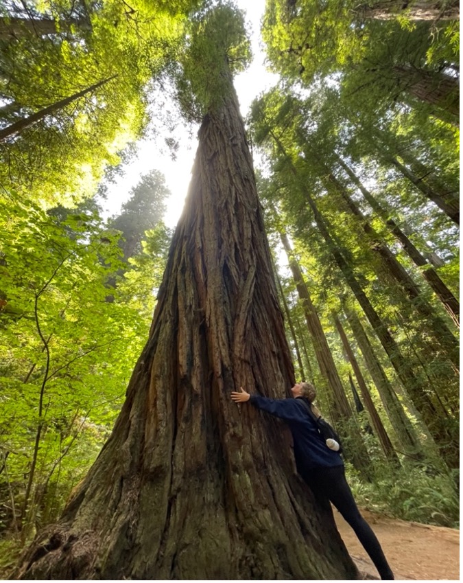
I have found the pattern of speeding up and slowing down are parallels outside of field work as well. In Port Orford specifically, slowing down has felt just as invigorating as the first breath one takes out of the water. For instance, the daily choice we make to squeeze 5 scientists into the world’s slowest elevator down to the lab every morning may not be practical in everyday life, but the extra minute looking at each other’s sleepy faces sets the foundation for our “go” mode. We also sit down after a day of fieldwork, as a team, eating our 5th version of pasta and meatballs while we continue our Hunger Games movie marathon from the night prior. And we chose our “off-day” to stroll among nature’s gentle giants, experiencing together the awe of the Redwoods trees.
Fig 4A & 4B: (A) Team Protein (Sophia, Oceana, Allison, Eden and I) slow morning elevator ride down to the lab. (B) Sophia hugging a tree at the Redwoods!
When my manager asked the above question, I couldn’t help but think upon an excerpt, popularly known as “The Fig Tree” by Sylvia Plath.
Fig 5: The Fig Tree excerpt by Sylvia Plath. Picture credits to @samefacecollective on Instagram.
For my fig tree, I imagine it as grandiose as those Redwood trees. What makes each of us choose one fig over the other is highly variable, just as our figs of possibilities, some of which we can’t make out quite yet. At some point along my life, the fig of owning a restaurant in the Big Apple propped up. But in that moment with my manager, I imagined my oldest fig, with little Celest sitting on the living room floor watching ocean documentaries and wanting nothing more than to conduct whale research, now winking at me as I start my master’s within the GEMM Lab. Your figs might be different from mine but what I believe we share in common is the alternating pace toward our fig. At times we need speeding up while other times we just need slowing down.
Then there’s that sweet spot in between where we can experience both, just as I have being a part of the 2024 TOPAZ/JASPER team.
Fig 6A and 6B: (A) My sister and I excited to go see some dolphins for the first time! (~2008). (B) Taking undergraduate graduation pics with my favorite whale plushy! (2023)
Fig 7: Team Protein takes on Port Orford Minimal Carnival, lots of needed booging after finishing field work!
By Matoska Silva, OSU Department of Integrative Biology, CEOAS REU Program
My name is Matoska Silva, and I just finished my first year at Oregon State University studying biology with a focus in ecology. This summer will be my first experience with marine ecology, and I’m eager to dive right in. I’m super excited for the opportunity to research krill due to the huge impacts these tiny organisms have on their surrounding ecosystems. The two weeks I’ve spent in the CEOAS REU so far have been among the most fun and informative of my life, and I can’t wait to see what else the summer has in store for me.
Figure 1. Matoska presents his proposed research to the CEOAS REU program.
I’ve spent most of my life in Oregon, so I was thrilled to learn that my project would focus on krill distribution along the Oregon Coast that I know and love. More specifically, my project focuses on the Northern California Current (NCC, the current found along the Oregon Coast) and the ways that geographic distribution of krill corresponds to climatic conditions in the region. Here is a synopsis of the project:
The NCC system, which spans the west coast of North America from Cape Mendocino, California to southern British Columbia, is notable for seasonal upwelling, a process that brings cool, nutrient-rich water from the ocean depths to the surface. This process provides nutrients for a complex marine food web containing phytoplankton, zooplankton, fish, birds, and mammals (Checkley & Barth, 2009). Euphausiids, commonly known as krill, are among the most ecologically important zooplankton groups in the NCC, playing a vital role in the flow of nutrients through the food web (Evans et al., 2022). Euphausia pacifica and Thysanoessa spinifera are the predominant krill species in the NCC, with T. spinifera mainly inhabiting coastal waters and E. pacifica inhabiting a wider range offshore (Brinton, 1962). T. spinifera individuals are typically physically larger than E. pacifica and are generally a higher-energy food source for predators (Fisher et al., 2020).
Temperature has been previously established as a major factor impacting krill abundance and distribution in the NCC (Phillips et al., 2022). Massive, ecosystem-wide changes in the NCC have been linked to extreme warming brought on by the 2014-2016 marine heatwave (Brodeur et al., 2019). Both dominant krill species have been shown to respond negatively to warming events in the NCC, with anomalous warm temperatures in 2014-2016 being linked to severe declines in E. pacifica biomass and with T. spinifera nearly disappearing from the Oregon Coast (Peterson et al., 2017). Changes in normal seasonal size variation and trends toward smaller size distributions in multiple age groups have been observed in E. pacifica in response to warming in northern California coastal waters (Robertson & Bjorkstedt, 2020).
The El Niño-Southern Oscillation (ENSO) is a worldwide climatic pattern that has been linked to warming events and ecosystem disturbances in the California Current System (McGowan et al., 1998). El Niño events of both strong and weak intensity can result in changes in the NCC ecosystem (Fisher et al., 2015). Alterations in the typical zooplankton community accompanying warm water conditions and a decline in phytoplankton have been recorded in the NCC during weak and strong El Niño occurrences (Fisher et al., 2015). A strong El Niño event occurred in 2023 and 2024, with three-month Oceanic Niño Index means reaching above 1.90 from October 2023 to January 2024 (NOAA Climate Prediction Center, https://www.cpc.ncep.noaa.gov/data/indices/oni.ascii.txt).
Figure 2. A graph of the ONI showing variability across two decades. Retrieved from NOAA at https://www.climate.gov/news-features/understanding-climate/climate-variability-oceanic-nino-index
While patterns in krill responses to warming have been described from previous years, the effects of the 2023-2024 El Niño on the spatial distribution of krill off the Oregon coast have not yet been established. As climate models have predicted that strong El Niño events may become more common due to greenhouse warming effects (Cai et al., 2014), continuing efforts to document zooplankton responses to El Niño conditions are vital for understanding how the NCC ecosystem responds to a changing climate. By investigating krill spatial distributions in April 2023, during a period of neutral ENSO conditions following a year of La Niña conditions, and April 2024, during the 2023-2024 El Niño event, we can assess how recent ENSO activity has impacted krill distributions in the NCC. In addition to broader measures of ENSO, we will examine records of localized sea surface temperatures (SST) and measurements of upwelling activity during April 2023 and 2024.
Understanding spatial distribution of krill aggregations is both ecologically and economically relevant, with implications for both marine conservation and management of commercial fisheries. Modeling patterns in the distribution of krill species and their predators has potential to inform marine management decisions to mitigate human impacts on marine mammals like whales (Rockwood et al., 2020). The data used to identify krill distribution were originally collected as part of the Marine Offshore Species Assessments to Inform Clean Energy (MOSAIC) project. The larger MOSAIC initiative centers around monitoring marine mammals and birds in areas identified for possible future development of offshore wind energy infrastructure. The findings of this study could aid in the conservation of krill consumers during the implementation of wind energy expansion projects. Changes in krill spatial distribution are also important for monitoring species that support commercial fisheries. Temperature has been shown to play a role in the overlap in distribution of NCC krill and Pacific hake (Merluccius productus), a commercially valuable fish species in Oregon waters (Phillips et al., 2023). The findings of my project could supplement existing commercial fish abundance surveys by providing ecological insights into factors driving changes in economically important fisheries.
Figure 3. The study area and transect design of the MOSAIC project, during which active acoustic data was collected (MOSAIC Project, https://mmi.oregonstate.edu/marine-mammals-offshore-wind).
I’m very grateful for the chance to work on a project with such important implications for the future of our Oregon coast ecosystems. My project has a lot of room for additional investigation of climate variables, with limited time being the main constraint on which processes I can explore. There are also unique methodological challenges to address during the project, and I’m ready to do some experimentation to work out solutions. Wherever my project takes me, I know that I will have developed a diverse range of skills and knowledge of krill by the end of the summer.
References
Brinton, E. (1962). The distribution of Pacific euphausiids. Bulletin of the Scripps Institution of Oceanography, 8(2), 51-270. https://escholarship.org/uc/item/6db5n157
Brodeur, R. D., Auth, T. D., & Phillips, A. J. (2019). Major shifts in pelagic micronekton and macrozooplankton community structure in an upwelling ecosystem related to an unprecedented marine heatwave. Frontiers in Marine Science, 6. https://doi.org/10.3389/fmars.2019.00212
Cai, W., Borlace, S., Lengaigne, M., van Rensch, P., Collins, M., Vecchi, G., Timmermann, A., Santoso, A., McPhaden, M. J., Wu, L., England, M. H., Wang, G., Guilyardi, E., & Jin, F. F. (2014). Increasing frequency of extreme El Niño events due to greenhouse warming. Nature Climate Change, 4, 111–116. https://doi.org/10.1038/nclimate2100
Checkley, D. M., & Barth, J. A. (2009). Patterns and processes in the California Current System. Progress in Oceanography, 83, 49–64. https://doi.org/10.1016/j.pocean.2009.07.028
Evans, R., Gauthier, S., & Robinson, C. L. K. (2022). Ecological considerations for species distribution modelling of euphausiids in the Northeast Pacific Ocean. Canadian Journal of Fisheries and Aquatic Sciences, 79, 518–532. https://doi.org/10.1139/cjfas-2020-0481
Fisher, J. L., Peterson, W. T., & Rykaczewski, R. R. (2015). The impact of El Niño events on the pelagic food chain in the northern California Current. Global Change Biology, 21, 4401–4414. https://doi.org/10.1111/gcb.13054
Fisher, J. L., Menkel, J., Copeman, L., Shaw, C. T., Feinberg, L. R., & Peterson, W. T. (2020). Comparison of condition metrics and lipid content between Euphausia pacifica and Thysanoessa spinifera in the Northern California Current, USA. Progress in Oceanography, 188, 102417. https://doi.org/10.1016/j.pocean.2020.102417
McGowan, J. A., Cayan, D. R., & Dorman, L. M. (1998). Climate-ocean variability and ecosystem response in the Northeast Pacific. Science, 281, 210–217. https://doi.org/10.1126/science.281.5374.210
Phillips, E. M., Chu, D., Gauthier, S., Parker-Stetter, S. L., Shelton, A. O., & Thomas, R. E. (2022). Spatiotemporal variability of Euphausiids in the California Current Ecosystem: Insights from a recently developed time series. ICES Journal of Marine Science, 79, 1312–1326. https://doi.org/10.1093/icesjms/fsac055
Phillips, E. M., Malick, M. J., Gauthier, S., Haltuch, M. A., Hunsicker, M. E., Parker‐Stetter, S. L., & Thomas, R. E. (2023). The influence of temperature on Pacific hake co‐occurrence with euphausiids in the California Current Ecosystem. Fisheries Oceanography, 32, 267–279. https://doi.org/10.1111/fog.12628
Peterson, W. T., Fisher, J. L., Strub, P. T., Du, X., Risien, C., Peterson, J., & Shaw, C. T. (2017). The pelagic ecosystem in the Northern California Current off Oregon during the 2014–2016 warm anomalies within the context of the past 20 years. Journal of Geophysical Research: Oceans, 122(9), 7267–7290. https://doi.org/10.1002/2017jc012952
Robertson, R. R., & Bjorkstedt, E. P. (2020). Climate-driven variability in Euphausia pacificasize distributions off Northern California. Progress in Oceanography, 188, 102412.https://doi.org/10.1016/j.pocean.2020.102412
In case you aren’t already aware, I want to remind you of a website called IndividuWhale we created about Pacific Coast Feeding Group (PCFG) gray whales we study as part of our GRANITE project. IndividuWhale features stories of some of the Oregon coast’s most iconic gray whales, as well as information about how we study them, stressors they experience in our waters, and even a game to test your gray whale identification skills. We also provide details about where to best spot gray whales along our coast and the different behaviors you might see gray whales displaying at different times of the year. Since launching the website in late 2021, we have made small tweaks and updates along the way, but now, after about 2.5 years, the time has come for a major content update as we are introducing you to three new individuals and their stories! Head over to IndividuWhale.com to check out the updates or continue reading for a preview of the content…
Lunita
Even though “Lunita” is only two years old (as of 2024), they (sex currently unknown!) have quickly become a star of our dataset and hearts. We documented Lunita as a calf with their mother “Luna” (hence the name Lunita, which means little Luna/moon) in 2022. We observed the mom-calf pair in our study area for almost two weeks during which it seemed like Lunita was a very attentive calf, always staying close to Luna and appearing to benthic feed alongside their mom. As is often the case when we document mom–calf pairs, we wonder whether we will see the calf again and how it will fair in an environment increasingly impacted by human activities. Much to our delight, we were reunited with Lunita later in the same summer when we saw them feeding independently, indicating that they had successfully weaned. We were even more delighted when we were reunited with Lunita again many times during the summer of 2023 as Lunita spent almost the entire feeding season along the central Oregon coast. This is yet another example, much like “Cheetah” and “Pacman,” of successful internal recruitment of calves born to PCFG females into the PCFG sub-population.
Lunita’s high site fidelity to our study area in 2023 meant that she was an excellent candidate for the suction-cup tagging we have been conducting in the last few years. During suction-cup tagging, we attach a device (or tag) via suction cups to a whale’s back. The tag contains a number of different sensors, including an accelerometer (to measure speed), a gyroscope (to measure direction), and a magnetometer (to measure magnetic field), as well as a high-definition video camera and hydrophone (or underwater microphone). These tags typically stay on for a maximum of 24 hours before they pop off the whale leaving no harm to the whale. Upon retrieval, we can recreate the whale’s dive path and see the environment and conditions that the whale experienced over several hours. We sometimes refer to tagging as giving the gray whales some temporary jewelry because the tags are a very flashy, bright orange color. From the video from Lunita’s tag shows how they soared through kelp forests feeding on mysids for many, many hours. Check out their profile here: https://www.individuwhale.com/whales/lunita/
Burned
There are many ways to assess the health of a whale. In our lab, we calculate body condition from drone images to determine how fat or skinny a whale is, examine different hormones from their poop, and assess growth rates via length measurements from drone images. Another health assessment metric that we explore in the lab is the skin and scarring on the individuals that we see in our central Oregon study area. By conducting a skin and scarring analysis, we can identify scarring patterns and lesions that may indicate interactions with human activities and track the progression of skin diseases that will help us understand the prevalence and impacts of pathogens on whales. One skin condition that we are particularly interested in tracking appears as a thick white or gray layer that can mask a gray whale’s natural pigmentation. An example of a whale that has experienced this skin condition is “Burned.”
Burned is a female who is at least 9 years old (as of 2024), as she was first documented in the PCFG range in 2015. We saw Burned for the first time in 2016. At the time, we noticed small, isolated, gray patches of the skin condition on both sides of Burned’s body. Throughout the years as we have continued to resight Burned, we noticed the skin condition spreading progressively across her body. We saw the skin condition at its maximum extent in 2022 when, at first glance, Burned was hardly recognizable. Luckily, we can identify gray whales using more than just their pigmentation patterns (learn more on our whale identification page). Interestingly, when we saw Burned in June 2024, it appeared that the skin condition completely disappeared! Burned is just one example of whales with this skin condition, leaving us with many questions about its origin and impact on the whales: What causes the skin condition (viral, fungal, bacterial?); How it is transmitted (via air or contact?); Is it harmful to the whale (weakened immune system?). Our research is aimed at addressing these questions to make this skin condition a little less mysterious. Check out her profile here: https://www.individuwhale.com/whales/burned/
Heart
“Heart,” who is also known as “Ginger,” is a very well known and popular whale in the Depoe Bay region. Heart is a female who is particularly famous for being a “tall fluker,” meaning that when she dives, she arches her tail fluke high in the air before it glides elegantly into the water. Heart was first documented as a calf in 2010, which means that she is 14 years old (as of 2024). At 14 years of age, we would expect for Heart to have had at least one, if not more, calves by now, as it is believed that gray whales reach sexual maturity at age 8 or 9. However, Heart has never been documented with a calf. Why?
While we cannot know for sure, we have a theory that it might be linked to her body length. Recent work in our lab has explored how growth of PCFG whales has changed over time. Using measurements of whales from our drone data, we investigated how the asymptotic length (i.e. the final length reached once an individual stops growing) for the PCFG whales has changed since the 1980s. Shockingly, we found that starting in the year 2000 the asymptotic length of PCFG whales has declined at an average rate of 0.05–0.12 meters per year. Over time, this means that a whale born in 2020 is expected to reach an adult body length that is 13% shorter than a gray whale born prior to 2000. In Heart’s case specifically, when we last measured her length at 13 years old, she was 10.65 meters long. If she had been born prior to 2000, then she would be 12.04 meters long by now at the age of 13. That’s a whole 1.5 meters (or almost 5 feet) shorter!
You might be wondering how Heart’s length links back to her ability to have a calf. It takes a lot of energy to be pregnant and support the fetus, so by being smaller, Heart may not be able to store and allocate enough energy towards reproduction. Many of the whales we commonly see are shorter than expected based on their age (including “Zorro”), so we are monitoring the number and frequency of calves in the PCFG to see how this decline in length may impact the population. Check our her profile here: https://www.individuwhale.com/whales/heart/
Be sure to head over to IndividuWhale.com to explore all of the whale profiles and lots of other information that we have provided there about PCFG gray whales and how we study them here in Oregon waters!
Did you enjoy this blog? Want to learn more about marine life, research, and conservation? Subscribe to our blog and get a weekly message when we post a new blog. Just add your name and email into the subscribe box below.
Graduate school is an odd phase of life, at least in my experience. You spend years hyperfocused on a project, learning countless new skills – and the journey is completely unique to you. Unlike high school or undergrad, you are on your own timeline. While you may have peers on similar timelines, at the end of day your major deadlines and milestone dates are your own. This has struck me throughout my time in grad school, and I’ve been thinking about it a lot lately as I approach my biggest, and final milestone – defending my PhD!
I defend in just about two months, and to be honest, it’s very odd approaching a milestone like this alone. In high school and college, you count down to the end together. The feelings of anticipation, stress, excitement, and anticipatory grief that can accompany the lead-up to graduation are typically shared. This time, as I’m in an intense final push to the end while processing these emotions, most of the people around me are on their own unique timeline. At times grad school can feel quite lonely, but this journey would have been impossible without an incredible community of people.
A central contradiction of being a grad student is that your research is your own, but you need a variety of communities to successfully complete it. Your community of formal advisors, including your advisor and committee members, guide you along the way and provide feedback. Professors help you fill specific knowledge and skill gaps, while lab mates provide invaluable peer mentorship. Finally, fellow grad students share the experience and can celebrate and commiserate with you. I’ve also had the incredible fortune of having the community of the GRANITE team, and I’ve recently been reflecting on how special the experience has been.
To briefly recap, GRANITE stands for Gray whale Response to Ambient Noise Informed by Technology and Ecology (read this blog to learn more). This project is one of the GEMM lab’s long-running gray whale projects focused on studying gray whale behavior, physiology, and health to understand how whales respond to ocean noise. Given the many questions under this project, it takes a team of researchers to accomplish our goals. I have learned so much from being on the team. While we spend most of the year working on our own components, we have annual meetings that are always a highlight of the year. Our team is made up of ecologists, physiologists, and statisticians with backgrounds across a range of taxa and methodologies. These meetings are an incredible time to watch, and participate in, scientific collaboration in action. I have learned so much from watching experts critically think about questions and draw inspiration from their knowledge bases. It’s been a multi-year masterclass and a critically important piece of my PhD.
The GRANITE team during our first in person meeting
These annual meetings have also served as markers of the passage of time. It’s been fascinating to observe how our discussions, questions, and ideas have evolved as the project progressed. In the early years, our presentations shared proposed research and our conversations focused on working out how on earth we were going to tackle the big questions we were posing. In parallel, it was so helpful to work out how I was going to accomplish my proposed PhD questions as part of this larger group effort. During the middle years, it was fun to hear progress updates and to learn from watching others go through their process too. In grad school, it’s easy to feel like your setbacks and stumbles are failures that reflect your own incompetence, but working alongside and learning from these scientists has helped remind me that setbacks and stumbles are just part of the process. Now, in the final phase, as results abound, it feels extra exciting to celebrate with this team that has watched the work, and me grow, from the beginning.
The GRANITE team taking a beach walk after our second in person meeting.
We just wrapped up our last team meeting of the GRANITE project, and this year provided a learning experience in a phase of science that isn’t often emphasized in grad school. For graduate students, our work tends to end when we graduate. While we certainly think about follow-up questions to our studies, we rarely get the opportunity to follow through. In our final exams, we are often asked to think of next steps outside the constraints of funding or practicality, as a critical thinking exercise. But it’s a different skillset to dream up follow-up questions, and to then assess which of those questions are feasible and could come together to form a proposal. This last meeting felt like a cool full-story moment. From our earliest meetings determining how to answer our new questions, to now deciding what the next new questions are, I have learned countless lessons from watching this team operate.
The GRANITE team after our third in person meeting.
There are a few overarching lessons I’ll take with me. First and foremost, the value of patience and kindness. As a young scientist stumbling up the learning curve of many skills all at once, I am so grateful for the patience and kindness I’ve been shown. Second, to keep an open mind and to draw inspiration from anything and everything. Studying whales is hard, and we often need to take ideas from studies on other animals. Which brings me to my third takeaway, to collaborate with scientists from a wide range of backgrounds who can combine their knowledges bases with yours, to generate better research questions and approaches to answering them.
I am so grateful to have worked with this team during my final sprint to the finish. Despite the pressure of the end nearing, I’m enjoying moments to reflect and be grateful. I am grateful for my teachers and peers and friends. And I can’t wait to share this project with everyone.
P.S. Interested in tuning into my defense seminar? Keep an eye on the GEMM lab Instagram (@gemm_lab) for the details and zoom link.
Did you enjoy this blog? Want to learn more about marine life, research, and conservation? Subscribe to our blog and get a weekly alert when we make a new post! Just add your name into the subscribe box below!
The EMERALD project (Examining Marine mammal Ecology through Regional Assessment of Long-term Data) has reached a milestone with a recent publication detailing our findings on long-term gray whale distribution, abundance, and habitat use patterns (Barlow et al. 2024). The study is made possible by an incredible dataset. Every May-July since 1992, a team of observers surveyed the coastline between the Columbia River at the border between Oregon and Washington and San Francisco Bay, California for marbled murrelets, a seabird species of conservation concern. They drive a small vessel along pre-determined tracklines, and record observations of seabirds and marine mammals—not just marbled murrelets—and fortunately for us, that means there is a record of annual gray whale distribution and abundance patterns that spans over three decades.
The Crescent Coastal Research team collecting survey data. We are incredibly grateful to Craig Strong and the many folks who collected these valuable observations over the years!
We analyzed these valuable data using density surface modeling to better understand what drives gray whale distribution and abundance, what their habitat preferences are, and whether and how these occurrence patterns have changed over time. I am excited to share a few of our findings here!
Long-term, stable hotspots
The survey data revealed three main areas with consistently high gray whale density: the central Oregon Coast off Newport, Cape Blanco off Oregon’s south coast, and the mouth of the Klamath River in northern California. Despite fluctuations in how many whales were observed over the years, these areas have remained predicable hotspots for gray whales during their summer feeding season.
(A) Mean gray whale encounter rate (whales/kilometers surveyed) summarized by year, across all latitudes. (B) Mean gray whale encounter rate summarized by 1° latitude bin, across all years. White indicates times and locations with no survey effort. (C) Mean gray whale encounter rate summarized by year and 1° latitude bin. (D) Map of the study area, with region boundaries shown by the dashed lines, and major placenames denoted. Figure and caption reproduced from Barlow et al. 2024.
Key regional differences
Major features like prominent capes divide the California Current into different regions with distinct oceanographic characteristics. We found that gray whales showed different habitat preferences in the different regions. In the northern part of our study area between the Columbia River and Cape Blanco, we found that rocky bottom substrate was strongly related to areas of higher gray whale abundance, despite being far less available than soft, sandy bottom habitat. In the region between Cape Blanco and Cape Mendocino, gray whales were more abundant in areas south of prominent capes and in closer proximity to river estuaries.
Coastal upwelling and relaxation are key
Coastal upwelling—the process by which winds in the spring and summer push surface water offshore that is then replaced by cold, nutrient-rich water that is brought into the sunlight and drives an abundance of marine life—is a critically important influence in the oceanography, ecology, and biodiversity of our study region. But relaxation of those upwelling winds is also important for coastal species, as relaxation events allow the upwelled nutrients to be retained in the nearshore waters and enhance and aggregate local productivity and prey. We found that gray whale abundance was highest when there was a combination of both upwelling and relaxation events—a critical balance of “enough but not too much”—that seems to be optimal for gray whale feeding opportunities in nearshore waters.
You are what, where, and how you eat
Gray whales are incredibly flexible predators and have a wide range of prey items they are known to feed on. We found that throughout our study range, gray whales have different habitat preferences. As they spend their summers here to feed, these habitat preferences are linked to their foraging preferences. Off the central Oregon Coast, gray whales are known to feed on zooplankton that aggregate around rocky reefs and kelp forests (Hildebrand et al. 2022, 2024).
A gray whale surfaces in a patch of kelp, foraging around a rocky reef. UAS image credit: GEMM Lab.
Further south, in the region between Cape Blanco and Cape Mendocino that encompassed the long-term hotspot of gray whale sightings off the Klamath River, our models revealed different habitat preferences. In the soft-bottom habitat off the Klamath River, gray whales are known to do more benthic feeding, whereby they scoop up the seafloor and filter out the invertebrates in the sediment such as amphipods and cumaceans (Mallonée 1991, Jenkinson 2001).
A gray whale surfaces with a mouth full of muddy sediment, filtering out the invertebrate prey. UAS image credit: GEMM Lab.
These differences in regional habitat preferences and preferred prey likely relate to larger-scale phenomena as well. Indeed, when we looked at how gray whale abundance in different regions related to widespread warm or cool phases in the North Pacific Ocean, the responses differed by region. This aspect of the study indicates that what gray whales eat and where they forage influences how they respond to shifting environmental conditions and prey availability.
Conservation of an iconic nearshore predator
The unique mosaic of habitat characteristics throughout the Northern California Current summer feeding range of gray whales provides them the opportunity to gain the energetic stores they need to survive, reproduce, and migrate. Thus, the reliability of these resources has led them to return to these stable foraging hotspots year after year. Under climate change, one potential impact on upwelling systems is shifts in the intensity and location of upwelling (Bograd et al. 2023); in the Northern California Current, this could mean reduced relaxation events that we found are crucial for gray whales feeding in this habitat. Furthermore, these whales overlap with human activities such as vessel disturbance, entanglement and vessel strike risk, and ocean noise throughout the foraging season, and have to bear the consequences of these anthropogenic stressors (Sullivan & Torres 2018, Lemos et al. 2022, Pirotta et al. 2023) as they also navigate changing environmental conditions. Our study highlights the value of long-term monitoring to better understand present ecological patterns in the context of the past, which can be used to inform conservation management decisions for the future.
Did you enjoy this blog? Want to learn more about marine life, research, and conservation? Subscribe to our blog and get a weekly alert when we make a new post! Just add your name into the subscribe box below!
References
Barlow DR, Strong CS, Torres LG (2024) Three decades of nearshore surveys reveal long-term patterns in gray whale habitat use, distribution, and abundance in the Northern California Current. Sci Rep 14:9352.
Bograd SJ, Jacox MG, Hazen EL, Lovecchio E, Montes I, Pozo Buil M, Shannon LJ, Sydeman WJ, Rykaczewski RR (2023) Climate Change Impacts on Eastern Boundary Upwelling Systems. Ann Rev Mar Sci 15:1–26.
Hildebrand L, Derville S, Hildebrand I, Torres LG (2024) Exploring indirect effects of a classic trophic cascade between urchins and kelp on zooplankton and whales. Sci Rep 14.
Hildebrand L, Sullivan FA, Orben RA, Derville S, Torres LG (2022) Trade-offs in prey quantity and quality in gray whale foraging. Mar Ecol Prog Ser 695:189–201.
Jenkinson RS (2001) Gray whale (Eschrichtius robustus) prey availability and feeding ecology in Northern California, 1999-2000. Humboldt State University
Lemos L, Haxel J, Olsen A, Burnett JD, Smith A, Chandler TE, Nieukirk SL, Larson SE, Hunt KE, Torres LG (2022) Effects of vessel traffic and ocean noise on gray whale stress hormones. Sci Rep 12:1–13.
Mallonée JS (1991) Behaviour of gray whales (Eschrichtius robustus) summering off the northern California coast, from Patrick’s Point to Crescent City. Can J Zool 69:681–690.
Pirotta E, Fernandez Ajó A, Bierlich KC, Bird CN, Buck CL, Haver SM, Haxel JH, Hildebrand L, Hunt KE, Lemos LS, New L, Torres LG (2023) Assessing variation in faecal glucocorticoid concentrations in gray whales exposed to anthropogenic stressors. Conserv Physiol 11:coad082.
Sullivan FA, Torres LG (2018) Assessment of vessel disturbance to gray whales to inform sustainable ecotourism. J Wildl Manage 82:896–905.