Celest Sorrentino, Research Technician, Geospatial Ecology of Marine Megafauna Lab
Hello again GEMM Lab family. I write to you exactly a year after (okay maybe 361 days after but who’s counting…) from my previous blog post describing my 2022 summer working in the GEMM Lab as an NSF REU intern. Since then, so much has changed, and I can’t wait to fill you in on it.
In June I walked across the commencement stage at UC Santa Barbara, earning my BS in Ecology, Evolution, and Marine Biology and my minor in Italian language. A week later, I packed my bags and headed straight back to the lukewarm beaches of Newport, Oregon as a Research Technician in the GEMM Lab. I am incredibly fortunate to have been invited back to the OSU Marine Mammal Institute to lend a hand analyzing drone footage of gray whales collected back in March 2023 when Leigh and Clara went down to Baja California, as mentioned previously in Clara’s blog.

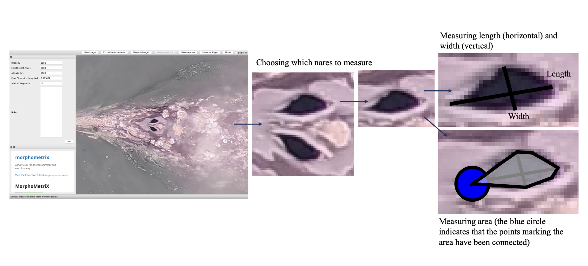
During my first meeting with Clara at the beginning of the summer we discussed that a primary goal of my position was to process all the drone footage collected in Baja so that the generated video clips could be later used in other analytical software such as BORIS and SLEAP A.I. Given my previous internships and past summer project, this video processing is familiar to me. My initial thoughts were:
Sweet! Watch drone footage, pop in some podcasts, note down when I see whales, let’s do this!*
Like any overly eager 23-year-old, I might have mentally cracked open a Celsius and kicked my feet up too soon. We added another layer to the goal: develop an ethogram – which requires me to identify and define the behaviors that the gray whales appear to be demonstrating within the videos (more on ethogram development in Clara’s previous blog.) This made me nervous.
I don’t have any experience with behavior. How do I tell what is a real behavior or if the whale is just existing? What if I’m wrong and ruin the project? What if I totally mess this up?
Naturally, as any sane person, to resolve these thoughts I took to the Reddit search bar: “How to do a job you’ve never done before.” No dice.
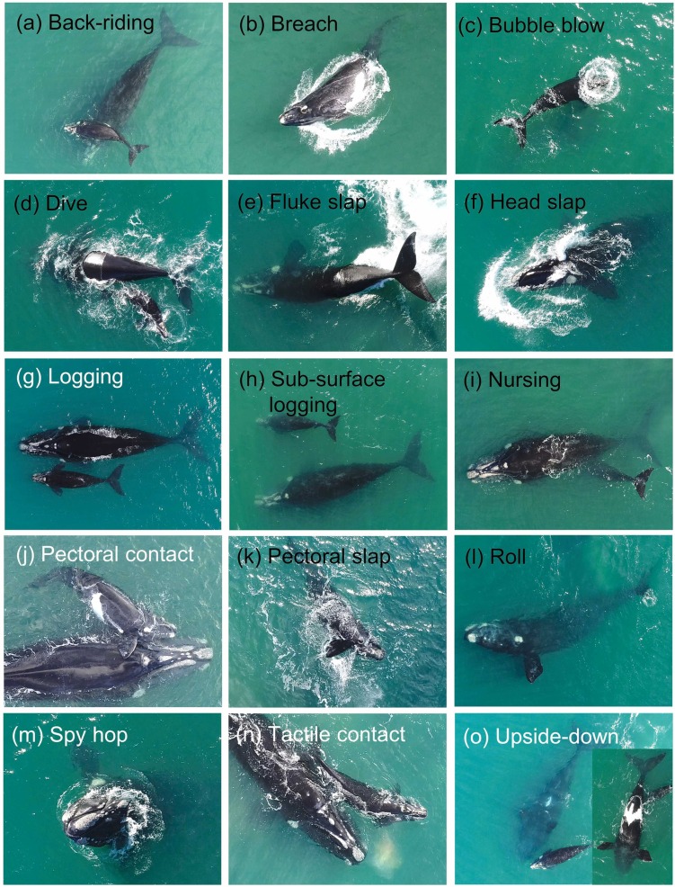
I pushed these thoughts aside and decided to just start the video analysis process. Clara provided me with the ethogram she is developing during her PhD as a point of reference (based on the published gray whale ethogram in Torres et al. 2018), I was surrounded by an insanely supportive lab, and I could Google anything at my fingertips. Fast-forward 6 weeks later: I had analyzed 128 drone videos of adult gray whales as well as mother-calf pairs, and developed an ethogram describing, 26 behaviors**. I named one of my favorite behaviors a “Twirl” to describe when a gray whale lifts their head out of the water and performs a 360 turn. Reminds me of times when as a kid, sometimes all you really needed is a good spin!
Now I was ready to start a productive, open conversation with Leigh and Clara about this ethogram and my work. However, even walking up to that last meeting, remnants of those daunting, doubtful early summer thoughts persisted. Even after I double checked all the definitions I wrote, rewatched all videos with said behaviors, and had something to show for my work. What gives Brain?
A few days ago, as I sat on my family’s living room couch with my two younger sisters, Baylie and Cassey, Baylie wanted to watch some TikToks with me. One video that came up was of a group of adults taking a beginner dance class, having so much fun and radiating joy. The caption read, Being a beginner as an adult is such a fun and wild thing. Baylie and I watched the video at least 10x, repeating to each other phrases like, “Wow!” and “They’re so cool.” That caption and video has been on my mind since:
Being a beginner as an adult is such a fun and wild thing.
Being a beginner as an adult is also scary.
Having just graduated, I can no longer say I am undergraduate student. Now, I am a young adult. This was my first research technician job, as an adult. Don’t adults usually have everything figured out? Can adults be beginners too?
Yes. In fact, we’re beginners more than we realize.
- I was a beginner cooking my mother’s turkey recipe 3 years ago for my housemates during the pandemic (Even after having her on Facetime, I still managed to broil it a little too long.)
- I was a beginner driver 5 years ago in a rickety Jeep driving myself to school (Now, since I’ve been back home, I’ve been driving my little sisters to school.)
- I was a beginner NSF REU intern just a year ago. (This summer I was the alumni on the panel for the current NSF REU interns at Hatfield.)
- I was a beginner science communicator presenting my NSF REU project at Hatfield last summer. (This summer, I presented my research at the Animal Behavior Society Conference.)


I now recognize that during my time identifying and defining behaviors of gray whales in videos made me take on the seat of a “beginner video and behavioral analyst”. I could not rely on the automated computer vision lens I gained from previous internships, which felt familiar and secure.
Instead, I had to allow myself to be creative. Dig into the unfamiliar in an effort to complete a task or job I had never done before. Allowing myself to be imperfect, make mistakes, meanwhile unconsciously building a new skill.
This is what makes being a beginner as an adult such a fun thing.
I don’t think being a beginner is a wild thing, although it can definitely make you feel a wild range of emotions. Being a beginner means you’re allowing yourself to try something new. Being a beginner means you’re allowing yourself the chance to learn.
Whether you’re an adult beginner as you enter your 30s, adult beginner as you enter parenthood, adult beginner grabbing a drink with friends after a long day in lab, adult beginner as a dancer, or like me, a beginner of leaving behind my college student persona and entering a new identity of adulthood, being a beginner as an adult is such a fun and normal thing.
I am not sure what will be next, but I hope to write to you all again from this blog a year from now, as an adult beginner as a grad student in the GEMM Lab. For anyone approaching the question of “What’s next”, I encourage you to read “Never a straight Path” by GEMM Lab MSc alum Florence Sullivan, a blog that has brought me such solace in my new adult journey and advice that never gets old.
Being a beginner—that, is so real.


*I listened to way too many podcasts to list them all, but I will include two that have been a GEMM Lab “gem” —-thanks to Lisa and Clara for looping me in and now, looping you in!)
- Serial Podcast(specifically Seasons 1-3)
- Operation Trade bomb
**(subject to change)
References
Torres LG, Nieukirk SL, Lemos L, Chandler TE (2018) Drone Up! Quantifying Whale Behavior From a New Perspective Improves Observational Capacity. Front Mar Sci 510.3389/fmars.2018.00319
Did you enjoy this blog? Want to learn more about marine life, research, and conservation? Subscribe to our blog and get a weekly message when we post a new blog. Just add your name and email into the subscribe box below.