By Hali Peterson, rising freshman, Western Oregon University
Hello, my name is Hali Peterson and I am a rising freshman in college. Last summer (2023) I was given the opportunity to be a paid high school intern for the OSU Marine Mammal Institute’s very own GEMM Lab (Geospatial Ecology of Marine Megafauna Laboratory) based at the Hatfield Marine Science Center in Newport, Oregon. My time working in the GEMM Lab has been supported by the Oregon Coast STEM Hub. I started my internship in June 2023 and I was one of the two GEMM Lab summer interns. However, my internship did not end when summer did, as I continued to work throughout the school year and even into this summer.

June 29, 2023 to September 20, 2024 (1 year, 2 months, and 21 days if anyone is curious) – what did I do and what did I learn during this time…
Initially, I was tasked with helping the GRANITE project (Gray whale Response to Ambient Noise Informed by Technology and Ecology) by processing drone footage of Pacific Coast Feeding Group (PCFG) gray whales and identifying their zooplankton prey. I started off my internship under the mentorship of KC Bierlich and Lisa Hildebrand and I dove into looking at zooplankton underneath a microscope and watching whales in drone footage, both gathered by the GEMM Lab field team.
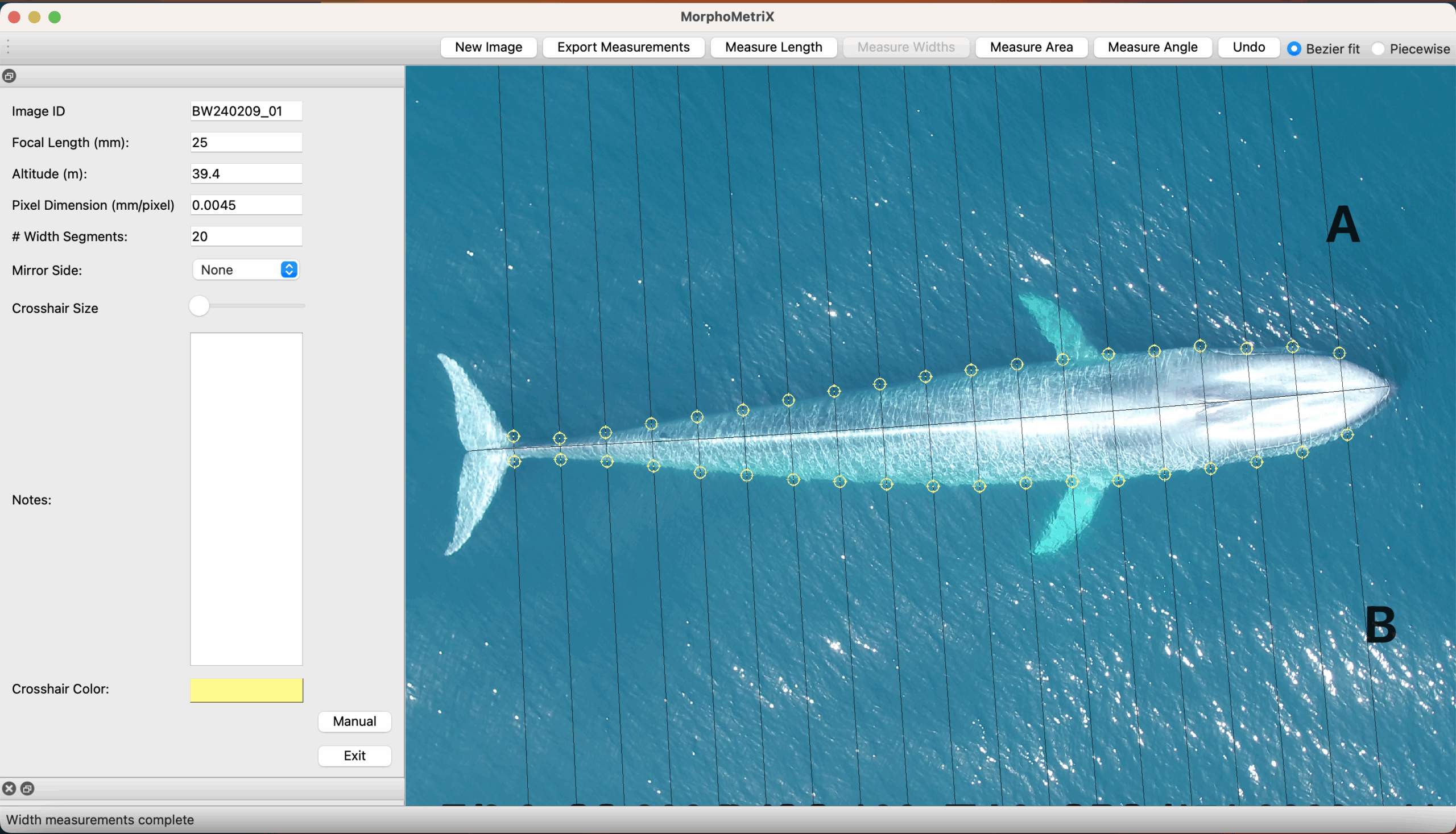
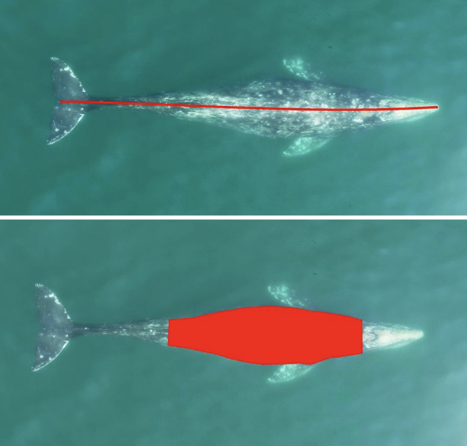
KC taught me how to process drone footage, measure whales and calibration boards, test an artificial intelligence model, as well as write a protocol of the drone processing methods that I had worked on. These tasks were a big responsibility as the measurements need to be accurate and precise so that they can be used to effectively assess the body condition of gray whales, which provides crucial insights into population health.

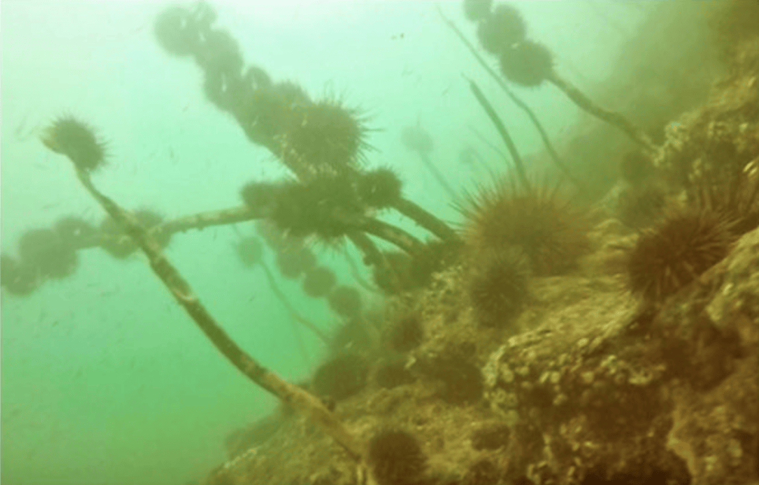
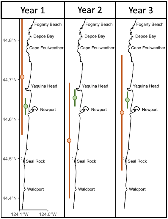
Under Lisa’s mentorship I learned how to identify and process zooplankton prey samples, process underwater GoPro videos, as well as identify and analyze kelp patches from satellite images. Within these tasks, I honed my expertise in zooplankton and habitat analysis and the results of my work will contribute to a deeper understanding of gray whale feeding habits along the Oregon coast.

As my main mentors, KC and Lisa taught me so much about the world of science and research. All of these detail-oriented and multi-layered tasks helped me improve some of the skills I already had before I started the internship as well as gift me with skills I didn’t previously possess. For example, I learned how to collaborate and work with a team, pay attention to detail, double and even triple check everything for quality work, problem solve, and learn to ask questions.
However, as my time in the GEMM Lab extended beyond the summer of 2023, so did my tasks. Later on I received another mentor, Clara Bird. Under Clara I learned how to identify whales from drone footage recorded in Baja, Mexico (an area that is specifically known as the breeding lagoons where the gray whales go in the winter), as well as use the Newport, Oregon drone footage and CATS (Customized Animal Tracking Solution) tag data to measure inhalation duration and bubble blast occurrences. These experiences furthered my knowledge and yet again I learned something new, a common theme throughout my time in the GEMM Lab.
Just a few months ago, the GEMM Lab hired Laura Flores Hernandez as a new high school student summer intern, and under the guidance of both Lisa Hildebrand and Leigh Torres, I was given the opportunity to develop my own mentoring skills. I used the skills I had obtained over the past year to teach someone else how to do the tasks I once was new to. I taught Laura how to identify zooplankton, process drone footage, and measure calibration boards. Stepping into that mentor role helped me reflect on my own learning and experiences. I had to go back and figure out how I did things, where I struggled, and how I overcame those struggles. Not an easy task but one I was glad to be presented with.

During my time here I was also invited to join a STEM (Science, Technology, Engineering, Mathematics) cruise led by Oregon Sea Grant with fellow high school students. On this science cruise I got to help look at box core samples (a tool used to collect large amounts of sediment off of the ocean floor). Equipped with my previous knowledge on zooplankton identification, I was able to help the chief scientist on the trip to explain to other high school students what we were seeing in the samples. This trip helped me grow my teamwork and identification skills, as well as experience what it is like to collect data while on a moving ship.

Another amazing opportunity I was selected for was to join the 2024 Girls on Icy Fjords team. This program, in association with OSU, was designed to empower young women in STEM in the backcountry of Alaska. With a team of 3 amazing instructors and 8 girls (all from different parts of the United States of America) we camped in the backcountry for 8 days, learning about glaciers and fjords, surviving in the backcountry, sea kayaking, and working as a team. I would highly recommend any young woman interested in science, art, or just an amazing experience to check out Inspiring Girls Expeditions.

All in all this will be a job that I will not soon forget; interning in the GEMM Lab has been both a learning opportunity as well as a challenge. My internship wasn’t without its challenges, from a computer that seemed determined to shut down whenever I made progress, to endless hours spent staring at a green screen, waiting to count a fish that might eventually swim by. Though the job had its ups and downs, I am so glad I was given this opportunity and was kept on in the lab for as long as I was. In just a few weeks, I will start my Bachelors of Aquarium Science at Western Oregon University and I’m both excited and nervous. I know that without a doubt the skills I learned during this internship will come in handy as I continue my education and pursue a career in the future.
Thank you to all my mentors, anyone who answered one of the many questions I had, and to the friends I made along the way!