Clara Bird, PhD Student, OSU Department of Fisheries, Wildlife, and Conservation Sciences, Geospatial Ecology of Marine Megafauna Lab
The start of a new school year is always an exciting time. Like high school, it means seeing friends again and the anticipation of preparing to learn something new. Even now, as a grad student less focused on coursework, the start of the academic year involves setting project timelines and goals, most of which include learning. As I’ve been reflecting on these goals, one of my dad’s favorite sayings has been at the forefront of my mind. As an overachieving and perfectionist kid, I often got caught up in the pursuit of perfect grades, so the phrase “just learn the stuff” was my dad’s reminder to focus on what matters. Getting good grades didn’t matter if I wasn’t learning. While my younger self found the phrase rather frustrating, I have come to appreciate and find comfort in it.
Given that my research is focused on behavioral ecology, I’ve also spent a lot of time thinking about how gray whales learn. Learning is important, but also costly. It involves an investment of energy (a physiological cost, Christie & Schrater, 2015; Jaumann et al., 2013), and an investment of time (an opportunity cost). Understanding the costs and benefits of learning can help inform conservation efforts because how an individual learns today affects the knowledge and tactics that the individual will use in the future.
Like humans, individual animals can learn a variety of tactics in a variety of ways. In behavioral ecology we classify the different types of learning based on the teacher’s role (even though they may not be consciously teaching). For example, vertical transmission is a calf learning from its mom, and horizontal transmission is an individual learning from other conspecifics (individuals of the same species) (Sargeant & Mann, 2009). An individual must be careful when choosing who to learn from because not all strategies will be equally efficient. So, it stands to reason than an individual should choose to learn from a successful individual. Signals of success can include factors such as size and age. An individual’s parent is an example of success because they were able to reproduce (Barrett et al., 2017). Learning in a population can be studied by assessing which individuals are learning, who they are learning from, and which learned behaviors become the most common.
An example of such a study is Barrett et al. (2017) where researchers conducted an experiment on capuchin monkeys in Costa Rica. This study centered around the Panama ́fruit, which is extremely difficult to open and there are several documented capuchin foraging tactics for processing and consuming the fruit (Figure 1). For this study, the researchers worked with a group of monkeys who lived in a habitat where the fruit was not found, but the group included several older members who had learned Panamá fruit foraging tactics prior to joining this group. During a 75-day experiment, the researchers placed fruits near the group (while they weren’t looking) and then recorded the tactics used to process the fruit and who used each tactic. Their results showed that the most efficient tactic became the most common tactic over time, and that age-bias was a contributing factor, meaning that individuals were more like to copy older members of the group.
Figure 1. Figure from Barrett et al. (2017) showing a capuchin monkey eating a Panamá fruit using the canine seam technique.
Social learning has also been documented in dolphin societies. A long-term study on wild bottlenose dolphins in Shark Bay, Australia assessed how habitat characteristics and the foraging behaviors used by moms and other conspecifics affected the foraging tactics used by calves (Sargeant & Mann, 2009). Interestingly, although various factors predicted what foraging tactic was used, the dominant factor was vertical transmission where the calf used the tactic learned from its mom (Figure 2). Overall, this study highlights the importance of considering a variety of factors because behavioral diversity and learning are context dependent.
Figure 2. Figure from Sargeant & Mann (2009) showing that the probability of a calf using a tactic was higher if the mother used that tactic.
Social learning is something that I am extremely interested in studying in our study population of gray whales in Oregon. While studies on social learning for such long-lived animals require a longer study period than of the span of our current dataset, I still find it important to consider the role learning may play. One day I would love to delve into the different factors of learning by these gray whales and answer questions such as those addressed in the studies I described above. Which foraging tactics are learned? How much of a factor is vertical transmission? Considering that gray whale calves spend the first few months of the foraging season with their mothers I would expect that there is at least some degree of vertical transmission present. Furthermore, how do environmental conditions affect learning? What tactics are learned in good vs. poor years of prey availability? Does it matter which tactic is learned first? While the chances that I’ll get to address these questions in the next few years are low, I do think that investigating how tactic diversity changes across age groups could be a good place to start. As I’ve discussed in a previous blog, my first dissertation chapter will focus on quantifying the degree of individual specialization present in my study group. After reading about age-biased learning, I am curious to see if older whales, as a group, use fewer tactics and if those tactics are the most energetically efficient.
The importance of understanding learning is related to that of studying individual specialization, which can allows us to estimate how behavioral tactics might change in popularity over time and space. We could then combine this with knowledge of how tactics are related to morphology and habitat and the associated energetic costs of each tactic. This knowledge would allow us to estimate the impacts of environmental change on individuals and the population. While my dissertation research only aims to provide a few puzzle pieces in this very large and complicated gray whale ecology puzzle, I am excited to see what I find. Writing this blog has both inspired new questions and served as a good reminder to be more patient with myself because I am still, “just learning the stuff”.
Dr. KC Bierlich, Postdoctoral Scholar, OSU Department of Fisheries, Wildlife, & Conservation Sciences, Geospatial Ecology of Marine Megafauna Lab
The morphology and body size of an animal is one of the most fundamental factors for understanding a species ecology. For instance, fish body size and fin shape can influence its habitat use, foraging behavior, prey type, physiological performance, and predator avoidance strategies (Fig 1). Morphology and body size can thus reflect details of an individual’s current health, likelihood of survival, and potential reproductive success, which directly influences a species life history patterns, such as reproductive status, growth rate, and energetic requirements. Collecting accurate morphological measurements of individuals is often essential for monitoring populations, and recent studies have demonstrated how animal morphology has profound implications for conservation and management decisions, especially for populations inhabiting anthropogenically-altered environments (Miles 2020) (Fig. 1). For example, in a study on the critically endangered European eel, De Meyer et al. (2020) found that different skulls sizes were associated with different ecomorphs (a local variety of a species whose appearance is determined by its ecological environment), which predicted different diet types and resulted with some ecomorphs having a greater exposure to pollutants and toxins than others. However, obtaining manual measurements of wild animal populations can be logistically challenging, limited by accessibility, cost, danger, and animal disturbance. These challenges are especially true for large elusive animals, such as whales that are often in remote locations, spend little time at the surface of the water, and their large size can preclude safe capture and live handling.
Figure 1. Top) A pathway framework depicting how the morphology of an animal influences its habitat use, behavior, foraging, physiology, and performance. These traits all affect how successful an animal is in its environment and can reflect an individual’s current health, likelihood of survival, and potential reproductive success. This individual success can then be scaled up to assess overall population health, which in turn can have direct implications for conservation. Bottom) an example of morphological differences in fish body size and fin shape from Walker et al. (2013). Fineness ratio (f) = length of body ÷ max body width.
Photogrammetry is a non-invasive method for obtaining accurate morphological measurements of animals from photographs. The two main types of photogrammetry methods used in wildlife biology are 1) single camera photogrammetry, where a known scale factor is applied to a single image to measure 2D distances and angles and 2) stereo-photogrammetry, where two or more images (from a single or multiple cameras) are used to recreate 3D models. These techniques have been used on domestic animals to measure body condition and estimate weight of dairy cows and lactating Mediterranean buffaloes (Negretti et al., 2008; Gaudioso et al., 2014) and on wild animals to measure sexual dimorphism in Western gorillas (Breuer et al., 2007), shoulder heights of elephants (Schrader et al., 2006), nutritional status of Japanese macaques (Kurita et al., 2012), and the body condition of brown bears (Shirane et al., 2020). Over 70 years ago, Leedy (1948) encouraged wildlife biologists to use aerial photogrammetry from aircraft for censusing wild animal populations and their habitats, where photographs can be collected at nadir (straight down) or an oblique angle, and the scale can be calculated by dividing the focal length of the camera by the altitude or by using a ratio of selected points in an image of a known size. Indeed, aerial photogrammetry has been wildly adopted by wildlife biologists and has proven useful in obtaining measurements in large vertebrates, such as elephants and whales.
Whitehead & Payne (1978) first demonstrated the utility of using aerial photogrammetry from airplanes and helicopters as a non-invasive technique for estimating the body length of southern right whales. Prior to this technique, measurements of whales were traditionally limited to assessing carcasses collected from scientific whaling operations, or opportunistically from commercial whaling, subsistence hunting, stranding events, and bycatch. Importantly, aerial photogrammetry provides a method to collect measurements of whales without killing them. This approach has been widely adopted to obtain body length measurements on a variety of whale and dolphin species, including bowhead whales (Cubbage & Calambokidis, 1987), southern right whales (Best & Rüther, 1992), fin whales (Ratnaswamy and Wynn, 1993), common dolphins (Perryman and Lynn, 1993), spinner dolphins (Perryman & Westlake 1998), and killer whales (Fearnbach et al. 2012). Aerial photogrammetry has also been used to measure body widths to estimate nutritive condition related to reproduction in gray whales (Perryman and Lynn, 2002) and northern and southern right whales (Miller et al., 2012). However, these studies collected photographs from airplanes and helicopters, which can be costly, limited by weather and infrastructure to support aircraft research efforts and, importantly, presents a potential risk to wildlife biologists (Sasse 2003).
The recent advancement and commercialization of unoccupied aircraft systems (UAS, or drones) has revolutionized the ability to obtain morphological measurements from high resolution aerial photogrammetry across a variety of ecosystems (Fig. 2). Drones ultimately bring five transformative qualities to conservation science compared to airplanes and helicopters: affordability, immediacy, quality, efficiency, and safety of data collection. Durban et al. (2015) first demonstrated the utility of using drones for non-invasively obtaining morphological measurements of killer whales in remote environments. Since then, drone-based morphological measurements have been applied to a wide range of studies that have increased our understanding on different whale populations. For example, Leslie et al. (2020) used drone-based measurements of the skull to distinguish a unique sub-species of blue whales off the coast of Chile. Groskreutz et al. (2019) demonstrated how long-term nutritional stress has limited body growth in northern resident killer whales, while Stewart et al. (2021) found a decrease in body length of North Atlantic Right whales since 1981 that was associated with entanglements from fishing gear and may be a contributing factor to the decrease in reproductive success for this endangered population.
Drone imagery is commonly used to estimate the body condition of baleen whales by measuring the body length and width of individuals. Recently, the GEMM Lab used body length and width measurements to quantify intra- and inter-seasonal changes in body condition across individual gray whales (Lemos et al., 2020). Drones have also been used to measure body condition loss in humpback whales during the breeding season (Christiansen et al., 2016) and to compare the healthy southern right whales to the skinnier, endangered North Atlantic right whales (Christiansen et al., 2020). Drone-based assessments of body condition have even been used to measure how calf growth rate is directly related to maternal loss during suckling (Christiansen et al., 2018), and even estimate body mass (Christiansen et al., 2019).
Drone-based morphological measurements can also be combined with whale-borne inertial sensing tag data to study the functional morphology across several different baleen whale species. Kahane-Rapport et al. (2020) used drone measurements of tagged whales to analyze the biomechanics of how larger whales require longer times for filtering the water through their baleen when feeding. Gough et al. (2019) used size measurements from drones and swimming speeds from tags to determine that a whale’s “walking speed” is 2 meters per second – whether the largest of the whales, a blue whale, or the smallest of the baleen whales, an Antarctic minke whale. Size measurements and tag data were combined by Segre et al. (2019) to quantify the energetic costs of different sized whales when breaching.
Taken together, drones have revolutionized our ability to obtain morphological measurements of whales, greatly increasing our capacity to better understand how these animals function and perform in their environments. These advancements in marine science are particularly important as these methods provide greater opportunity to monitor the health of populations, especially as they face increased threats from anthropogenic stressors (such as vessel traffic, ocean noise, pollution, fishing entanglement, etc.) and climate change.
Drone-based photogrammetry is one of the main focuses of the GEMM Lab’s project on Gray whale Response to Ambient Noise Informed by Technology and Ecology (GRANITE). This summer we have been collecting drone videos to measure the body condition of gray whales feeding off the coast of Newport, Oregon (Fig. 2). As we try to understand the physiological stress response of gray whales to noise and other potential stressors, we have to account for the impacts of overall nutritional state of each individual whale’s physiology, which we infer from these body condition estimates.
Figure 2. Drones can help collect images of whales to obtain morphological measurements using photogrammetry and help us fill knowledge gaps for how these animals interact in their environment and to assess their current health. Bottom photo is an image collected by the GEMM Lab of a gray whale being measured in MorphoMetriX software to estimate its body condition.
References
Best, P. B., & Rüther, H. (1992). Aerial photogrammetry of southern right whales, Eubalaena australis. Journal of Zoology, 228(4), 595-614.
Breuer, T., Robbins, M. M., & Boesch, C. (2007). Using photogrammetry and color scoring to assess sexual dimorphism in wild western gorillas (Gorilla gorilla). American Journal of Physical Anthropology, 134(3), 369–382. https://doi.org/10.1002/ajpa.20678
Christiansen, F., Vivier, F., Charlton, C., Ward, R., Amerson, A., Burnell, S., & Bejder, L. (2018). Maternal body size and condition determine calf growth rates in southern right whales. Marine Ecology Progress Series, 592, 267–281.
Christiansen, F. (2020). A population comparison of right whale body condition reveals poor state of North Atlantic right whale, 1–43.
Christiansen, F., Dujon, A. M., Sprogis, K. R., Arnould, J. P. Y., & Bejder, L. (2016). Noninvasive unmanned aerial vehicle provides estimates of the energetic cost of reproduction in humpback whales. Ecosphere, 7(10), e01468–18.
Christiansen, F., Sironi, M., Moore, M. J., Di Martino, M., Ricciardi, M., Warick, H. A., … Uhart, M. M. (2019). Estimating body mass of free-living whales using aerial photogrammetry and 3D volumetrics. Methods in Ecology and Evolution, 10(12), 2034–2044.
Cubbage, J. C., & Calambokidis, J. (1987). Size-class segregation of bowhead whales discerned through aerial stereo-photogrammetry. Marine Mammal Science, 3(2), 179–185.
De Meyer, J., Verhelst, P., & Adriaens, D. (2020). Saving the European Eel: How Morphological Research Can Help in Effective Conservation Management. Integrative and Comparative Biology, 23, 347–349.
Gaudioso, V., Sanz-Ablanedo, E., Lomillos, J. M., Alonso, M. E., Javares-Morillo, L., & Rodr\’\iguez, P. (2014). “Photozoometer”: A new photogrammetric system for obtaining morphometric measurements of elusive animals, 1–10.
Gough, W. T., Segre, P. S., Bierlich, K. C., Cade, D. E., Potvin, J., Fish, F. E., … Goldbogen, J. A. (2019). Scaling of swimming performance in baleen whales. Journal of Experimental Biology, 222(20), jeb204172–11.
Groskreutz, M. J., Durban, J. W., Fearnbach, H., Barrett-Lennard, L. G., Towers, J. R., & Ford, J. K. B. (2019). Decadal changes in adult size of salmon-eating killer whales in the eastern North Pacific. Endangered Species Research, 40, 1
Kahane-Rapport, S. R., Savoca, M. S., Cade, D. E., Segre, P. S., Bierlich, K. C., Calambokidis, J., … Goldbogen, J. A. (2020). Lunge filter feeding biomechanics constrain rorqual foraging ecology across scale. Journal of Experimental Biology, 223(20), jeb224196–8.
Leedy, D. L. (1948). Aerial Photographs, Their Interpretation and Suggested Uses in Wildlife Management. The Journal of Wildlife Management, 12(2), 191.
Lemos, L. S., Burnett, J. D., Chandler, T. E., Sumich, J. L., and Torres, L. G. (2020). Intra- and inter-annual variation in gray whale body condition on a foraging ground. Ecosphere 11.
Leslie, M. S., Perkins-Taylor, C. M., Durban, J. W., Moore, M. J., Miller, C. A., Chanarat, P., … Apprill, A. (2020). Body size data collected non-invasively from drone images indicate a morphologically distinct Chilean blue whale (Balaenoptera musculus) taxon. Endangered Species Research, 43, 291–304.
Miles, D. B. (2020). Can Morphology Predict the Conservation Status of Iguanian Lizards? Integrative and Comparative Biology.
Miller, C. A., Best, P. B., Perryman, W. L., Baumgartner, M. F., & Moore, M. J. (2012). Body shape changes associated with reproductive status, nutritive condition and growth in right whales Eubalaena glacialis and E. australis. Marine Ecology Progress Series, 459, 135–156.
Negretti, P., Bianconi, G., Bartocci, S., Terramoccia, S., & Verna, M. (2008). Determination of live weight and body condition score in lactating Mediterranean buffalo by Visual Image Analysis. Livestock Science, 113(1), 1–7. https://doi.org/10.1016/j.livsci.2007.05.018
Ratnaswamy, M. J., & Winn, H. E. (1993). Photogrammetric Estimates of Allometry and Calf Production in Fin Whales, \emph{Balaenoptera physalus}. American Society of Mammalogists, 74, 323–330.
Perryman, W. L., & Lynn, M. S. (1993). Idendification of geographic forms of common dolphin(\emph{Delphinus Delphis}) from aerial photogrammetry. Marine Mammal Science, 9(2), 119–137.
Perryman, W. L., & Lynn, M. S. (2002). Evaluation of nutritive condition and reproductive status of migrating gray whales (\emph{Eschrichtius robustus}) based on analysisof photogrammetric data. Journal Cetacean Research and Management, 4(2), 155–164.
Perryman, W. L., & Westlake, R. L. (1998). A new geographic form of the spinner dolphin, stenella longirostris, detected with aerial photogrammetry. Marine Mammal Science, 14(1), 38–50.
Sasse, B. (2003). Job-Related Mortality of Wildlife Workers in the United States, 1937- 2000, 1015–1020.
Segre, P. S., Potvin, J., Cade, D. E., Calambokidis, J., Di Clemente, J., Fish, F. E., … & Goldbogen, J. A. (2020). Energetic and physical limitations on the breaching performance of large whales. Elife, 9, e51760.
Shirane, Y., Mori, F., Yamanaka, M., Nakanishi, M., Ishinazaka, T., Mano, T., … Shimozuru, M. (2020). Development of a noninvasive photograph-based method for the evaluation of body condition in free-ranging brown bears. PeerJ, 8, e9982. https://doi.org/10.7717/peerj.9982
Shrader, A. M., M, F. S., & Van Aarde, R. J. (2006). Digital photogrammetry and laser rangefinder techniques to measure African elephants, 1–7.
Stewart, J. D., Durban, J. W., Knowlton, A. R., Lynn, M. S., Fearnbach, H., Barbaro, J., … & Moore, M. J. (2021). Decreasing body lengths in North Atlantic right whales. Current Biology.
Walker, J. A., Alfaro, M. E., Noble, M. M., & Fulton, C. J. (2013). Body fineness ratio as a predictor of maximum prolonged-swimming speed in coral reef fishes. PloS one, 8(10), e75422.
Clara Bird, PhD Student, OSU Department of Fisheries, Wildlife, and Conservation Sciences, Geospatial Ecology of Marine Megafauna Lab
When I thought about what doing fieldwork would be like, before having done it myself, I imagined that it would be a challenging, but rewarding and fun experience (which it is). However, I underestimated both ends of the spectrum. I simultaneously did not expect just how hard it would be and could not imagine the thrill of working so close to whales in a beautiful place. One part that I really did not consider was the pre-season phase. Before we actually get out on the boats, we spend months preparing for the work. This prep work involves buying gear, revising and developing protocols, hiring new people, equipment maintenance and testing, and training new skills. Regardless of how many successful seasons came before a project, there are always new tasks and challenges in the preparation phase.
For example, as the GEMM Lab GRANITE project team geared up for its seventh field season, we had a few new components to prepare for. Just to remind you, the GRANITE (Gray whale Response to Ambient Noise Informed by Technology and Ecology) project’s field season typically takes place from June to mid-October of each year. Throughout this time period the field team goes out on a small RHIB (rigid hull inflatable boat), whenever the weather is good enough, to collect photo-ID data, fecal samples, and drone imagery of the Pacific Coast Feeding Group (PCFG) gray whales foraging near Newport, OR, USA. We use the data to assess the health, ecology and population dynamics of these whales, with our ultimate goal being to understand the effect of ambient noise on the population. As previous blogs have described, a typical field day involves long hours on the water looking for whales and collecting data. This year, one of our exciting new updates is that we are going out on two boats for the first part of the field season and starting our season 10 days early (our first day was May 20th). These updates are happening because a National Science Foundation funded seismic survey is being conducted within our study area starting in June. The aim of this survey is to assess geophysical structures but provides us with an opportunity to assess the effect of seismic noise on our study group by collecting data before, during, and after the survey. So, we started our season early in order to capture the “before seismic survey” data and we are using a two-boat approach to maximize our data collection ability.
While this is a cool opportunistic project, implementing the two-boat approach came with a new set of challenges. We had to find a second boat to use, buy a new set of gear for the second boat, figure out the best way to set up our gear on a boat we had not used before, and update our data processing protocols to include data collected from two boats on the same day. Using two boats also means that everyone on the core field team works every day. This core team includes Leigh (lab director/fearless leader), Todd (research assistant), Lisa (PhD student), Ale (new post-doc), and me (Clara, PhD student). Leigh and Todd are our experts in boat driving and working with whales, Todd is our experienced drone pilot, I am our newly certified drone pilot, and Lisa, Ale, and myself are boat drivers. Something I am particularly excited about this season is that Lisa, Ale, and I all have at least one field season under our belts, which means that we get to become more involved in the process. We are learning how to trailer and drive the boats, fly the drones, and handling more of the post-field work data processing. We are becoming more involved in every step of a field day from start to finish, and while it means taking on more responsibility, it feels really exciting. Throughout most of graduate school, we grow as researchers as we develop our analytical and writing skills. But it’s just as valuable to build our skillset for field work. The ocean conditions were not ideal on the first day of the field season, so we spent our first day practicing our field skills.
For our “dry run” of a field day, we went through the process of a typical day, which mostly involved a lot of learning from Leigh and Todd. Lisa practiced her trailering and launching of the boat (figure 1), Ale and Lisa practiced driving the boat, and I practiced flying the drone (figure 2). Even though we never left the bay or saw any whales, I thoroughly enjoyed our dry run. It was useful to run through our routine, without rushing, to get all the kinks out, and it also felt wonderful to be learning in a supportive environment. Practicing new skills is stressful to say the least, especially when there is expensive equipment involved, and no one wants to mess up when they’re being watched. But our group was full of support and appreciation for the challenges of learning. We cheered for successful boat launchings and dockings, and drone landings. I left that day feeling good about practicing and improving my drone piloting skills, full of gratitude for our team and excited for the season ahead.
Figure 1. Lisa (driving the truck) launching the boat.
Figure 2. Clara (seated, wearing a black jacket) landing the drone in Ale’s hands.
All the diligent prep work paid off on Saturday with a great first day (figure 3). We conducted five GoPro drops (figure 4), collected seven fecal samples from four different whales (figure 5), and flew four drone flights over three individuals including our star from last season, Sole. Combined, we collected two trifectas (photo-ID images, fecal samples, and drone footage)! Our goal is to get as many trifectas as possible because we use them to study the relationship between the drone data (body condition and behavior) and the fecal sample data (hormones). We were all exhausted after 10 hours on the water, but we were all very excited to kick-start our field season with a great day.
Figure 3. Lisa on the bow pulpit during our first sighting of the day.
Figure 4. Lisa doing a GoPro drop, she’s lowering the GoPro into the water using the line in her hands.
Figure 5. Clara and Ale collecting a fecal sample.
On Sunday, just one boat went out to collect more data from Sole after a rainy morning and I successfully flew over her from launching to landing! We have a long season ahead, but I am excited to learn and see what data we collect. Stay tuned for more updates from team GRANITE as our season progresses!
Clara Bird, PhD Student, OSU Department of Fisheries and Wildlife, Geospatial Ecology of Marine Megafauna Lab
In order to understand a species’ distribution, spatial ecologists assess which habitat characteristics are most often associated with a species’ presence. Incorporating behavior data can improve this analysis by revealing the functional use of each habitat type, which can help scientists and managers assign relative value to different habitat types. For example, habitat used for foraging is often more important than habitat that a species just travels through. Further complexity is added when we consider that some species, such as gray whales, employ a variety of foraging tactics on a variety of prey types that are associated with different habitats. If individual foraging tactic specialization is present, different foraging habitats could be valuable to specific subgroups that use each tactic. Consequently, for a population that uses a variety of foraging tactics, it’s important to study the associations between tactics and habitat characteristics.
Lukoschek and McCormick’s (2001) study investigating the spatial distribution of a benthic fish species’ foraging behavior is a great example of combining data on behavior, habitat, and morphology. They collected data on the diet composition of individual fish categorized into different size classes (small, medium, and large) and what foraging tactics were used in which reef zones and habitat types. The foraging tactics ranged from feeding in the water column to digging (at a range of depths) in the benthic substrate. The results showed that an interesting combination of fish behavior and morphology explained the observed diet composition and spatial distribution patterns. Small fish foraged in shallower water, on smaller prey, and primarily employed the water column and shallow digging tactics. In contrast, large fish foraged in deep water, on larger prey, and primarily fed by digging deeper into the seafloor (Figure 1). This pattern is explained by both morphology and behavior. Morphologically, the size of the feeding apparatus (mouth gape size) affects the size of the prey that a fish can feed on. The gape of the small fish is not large enough to eat the larger prey that large fish are able to consume. Behaviorally, predation risk also affects habitat selection and tactic use. Small fish are at higher risk of being predated on, so they remain in shallow areas where they are more protected from predators and they don’t dig as deep to forage because they need to be able to keep an eye out for predators. Interestingly, while they found a relationship between the morphology of the fish and habitat use, they did not find an association between specific feeding tactics and habitat types.
Figure 1. Figure from Lukoschek and McCormick (2001) showing that small fish (black bar) were found in shallow habitat while large fish (white bar) were found in deep habitat.
Conversely, Torres and Read (2009) did find associations between theforaging tactics of bottlenose dolphins in Florida Bay, FL and habitat type. Dolphins in this bay employ three foraging tactics: herd and chase, mud ring feeding, and deep diving. Observations of the foraging tactics were linked to habitat characteristics and individual dolphins. The study found that these tactics are spatially structured by depth (Figure 2), with deep diving occurring in deep water whereas mud ring feeding occurrs in shallower water. They also found evidence of individual specialization! Individuals that were observed deep diving were not observed mud ring feeding and vice-versa. Furthermore, they found that individuals were found in the habitat type associated with their preferred tactic regardless of whether they were foraging or not. This result indicates that individual dolphins in this bay have a foraging tactic they prefer and tend to stay in the corresponding habitat type. These findings are really intriguing and raise interesting questions regarding how these tactics and specializations are developed or learned. These are questions that I am also interested in asking as part of my thesis.
Figure 2. Figure from Torres and Read (2009) showing that deep diving is associated with deeper habitat while mud ring feeding is associated with shallow habitat.
Both of these studies are cool examples that, combined, exemplify questions I am interested in examining using our study population of Pacific Coast Feeding Group (PCFG) gray whales. Like both studies, I am interested in assessing how specific foraging tactics are associated with habitat types. Our hypothesis is that different prey types live in different habitat types, so each tactic corresponds to the best way to feed on that prey type in that habitat. While predation risk doesn’t have as much of an effect on foraging gray whales as it does on small benthic fish, I do wonder how disturbance from boats could similarly affect tactic preference and spatial distribution. I am also curious to see if depth has an effect on tactic choice by using the morphology data from our drone-based photogrammetry. Given that these whales forage in water that is sometimes as deep as they are long, it stands to reason that maneuverability would affect tactic use. As described in a previous blog, I’m also looking for evidence of individual specialization. It will be fascinating to see how foraging preference relates to space use, habitat preference, and morphology.
These studies demonstrate the complexity involved in studying a population’s relationship to its habitat. Such research involves considering the morphology and physiology of the animals, their social, individual, foraging, and predator-prey behaviors, and the relationship between their prey and the habitat. It’s a bit daunting but mostly really exciting because better understanding each puzzle piece improves our ability to estimate how these animals will react to changing environmental conditions.
While I don’t have any answers to these questions yet, I will be working with a National Science Foundation Research Experience for Undergraduates intern this summer to develop a habitat map of our study area that will be used in this analysis and potentially answer some preliminary questions about PCFG gray whale habitat use patterns. So, stay tuned to hear more about our work this summer!
References
Lukoschek, V., & McCormick, M. (2001). Ontogeny of diet changes in a tropical benthic carnivorous fish, Parupeneus barberinus (Mullidae): Relationship between foraging behaviour, habitat use, jaw size, and prey selection. Marine Biology, 138(6), 1099–1113. https://doi.org/10.1007/s002270000530
Torres, L. G., & Read, A. J. (2009). Where to catch a fish? The influence of foraging tactics on the ecology of bottlenose dolphins ( Tursiops truncatus ) in Florida Bay, Florida. Marine Mammal Science, 25(4), 797–815. https://doi.org/10.1111/j.1748-7692.2009.00297.x
Clara Bird, PhD Student, OSU Department of Fisheries and Wildlife, Geospatial Ecology of Marine Megafauna Lab
When I started working on my thesis, I anticipated many challenges related to studying the behavioral ecology of gray whales. From processing five-plus years of drone footage to data analysis, there has been no shortage of anticipated and unexpected issues. I recently hit an unexpected challenge when I started video processing that piqued my interest. As I’ve discussed in a previous blog, ethograms are lists of defined behaviors that help us properly and consistently collect data in a standardized approach. Ethograms form a crucial foundation of any behavior study as the behaviors defined ultimately affect what questions can be asked and what patterns are detected. Since I am working off of the thorough ethogram of Oregon gray whales from Torres et al. (2018), I had not given much thought to the process of adding behaviors to the ethogram. But, while processing the first chunk of drone videos, I noticed some behaviors that were not in the original ethogram and struggled to decide whether or not to add them. I learned that ethogram development can lead down several rabbit holes. The instinct to try and identify every movement is strong but dangerous. Every minute movement does not necessarily need to be included and it’s important to remember the ultimate goal of the analysis to avoid getting bogged down.
Fundamental behavior questions cannot be answered without ethograms. For example, Baker et al. (2017) developed an ethogram for bottlenose dolphins in Ireland in order to conduct an initial quantitative behavior analysis. They did so by reviewing published ethograms for bottlenose dolphins, consulting with multiple experts, and revising the ethogram throughout the study. They then used their data to test inter-observer variability, calculate activity budgets, and analyze how the activity budgets varied across space and time.
Howe et al. (2015) also developed an ethogram in order to conduct quantitative behavior analyses. Their goals were to use the ethogram and subsequent analyses to better understand the behavior of beluga whales in Cook Inlet, AK, USA and to inform conservation. They started by writing down all behaviors they observed in the field, then they consolidated their notes into a formal ethogram that they used and refined during subsequent field seasons. They used their data to analyze how the frequencies of different behaviors varied throughout the study area at different times. This study served as an initial analysis investigating the effect of anthropogenic disturbance and was refined in future studies.
My research is similarly geared towards understanding behavior patterns to ultimately inform conservation. The primary questions of my thesis involve individual specialization, patterns of behavior across space, the relationship between behavior and body condition, and social behavior (check out this blog to learn more). While deciding what behaviors to add to my ethogram I’ve had to remind myself of these main questions and the bigger picture. The drone footage lets us see so much detail that it’s tempting to try to define every movement we can observe. One rabbit hole I’ve had to avoid a few times is locomotion. From the footage, it is possible to document fluke beats and pectoral fin strokes. While it could be interesting to investigate how different whales move in different ways, it could easily become a complicated mess of classifying different movements and take me deep into the world of whale locomotion. Talking through what that work would look like reminded me that we cannot answer every question and trying to assess all exciting side projects can cause us to lose focus on the main questions.
While I avoided going down the locomotion rabbit hole, there were some new behaviors that I did add to my ethogram. I’ll illustrate the process with the examples of two new behaviors I recently added: fluke swish and pass under (Clips 1 and 2). Clip 1 shows a whale rapidly moving its fluke to the side. I chose to add fluke swish because it’s such a distinct movement and I’m curious to see if there’s a pattern across space, time, individual, or nearby human activity that might explain its function. Clip 2 shows a calf passing under its mom. It’s not nursing because the calf doesn’t spend time under its mom, it just crosses underneath her. The calf pass under behavior could be a type of mom-calf tactile interaction. Analyzing how the frequency of this behavior changes over time could show how a calf’s dependency on its mom changes over as it ages.
In defining these behaviors, I had to consider how many different variations of this behavior would be included in the definition. This process involves considering at what point a variation of that behavior could serve a different function, even without knowing the function of the original behavior. For fluke swish this process involved deciding to only count a behavior as a fluke swish if it was a big, fast movement. A small and slow movement of the fluke a little to the side could serve a different function, such as turning, or be a random movement.
Clip 1: Fluke swish behavior (Video filmed under NOAA/NMFS research permit #16111 by certified drone pilot Todd Chandler).
Clip 2: Pass under behavior (Video filmed under NOAA/NMFS research permit #16111 by certified drone pilot Todd Chandler).
The next step involved deciding if the behavior would be a ‘state’ or ‘point’ event. A state event is a behavior with a start and stop moment; a point event is instantaneous and assigned to just a point in time. I would categorize a behavior as a state event if I was interested in questions about its duration. For example, I could ask “what percentage of the total observation time was spent in a certain behavior state?” A point event would be a behavior where duration is not applicable, but I could ask a question like “Did whale 1 perform more point event A than whale 2?”. Both fluke swish and pass under are point events because they only happen for an instant. In a pass under the calf is passing under its mom for just a brief point in time, making it a point event. The final step was to name the behavior. As I discussed in this blog, the name of the behavior does not matter as much as the definition but it is important that the name is clear and descriptive. We chose the name fluke swish because the fluke rapidly moves from side to side and pass under because the calf crosses under its mom.
Frankly, in the beginning, I was a bit overwhelmed by the realization that the content of my ethogram would ultimately control the questions I could answer. I could not help but worry that after processing all the videos, I would end up regretting not defining more behaviors. However, after reading some of the literature, chatting with Leigh, and reviewing the initial chunk of videos several times, I am more confidence in my judgment and my ethogram. I have accepted the fact that I can’t anticipate everything, and I am confident that the behaviors I need to answer my research questions are included. The process of reviewing and updating my ethogram has been a rewarding challenge that resulted in a valuable lesson that I will take with me for the rest of my career.
References
Baker, I., O’Brien, J., McHugh, K., & Berrow, S. (2017). An ethogram for bottlenose dolphins (Tursiops truncatus) in the Shannon Estuary, Ireland. Aquatic Mammals, 43(6), 594–613. https://doi.org/10.1578/AM.43.6.2017.594
Howe, M., Castellote, M., Garner, C., McKee, P., Small, R. J., & Hobbs, R. (2015). Beluga, Delphinapterus leucas, ethogram: A tool for cook inlet beluga conservation? Marine Fisheries Review, 77(1), 32–40. https://doi.org/10.7755/MFR.77.1.3
Torres, L. G., Nieukirk, S. L., Lemos, L., & Chandler, T. E. (2018). Drone up! Quantifying whale behavior from a new perspective improves observational capacity. Frontiers in Marine Science, 5(SEP). https://doi.org/10.3389/fmars.2018.00319
Clara Bird, PhD Student, OSU Department of Fisheries and Wildlife, Geospatial Ecology of Marine Megafauna Lab
As anyone who has ever been, or raised, a picky eater knows, humans have a wide range of food preferences. The diversity of available cuisines is a testament to the fact that we have individual food preferences. While taste is certainly a primary influence, nutritional benefits and accessibility are other major factors that affect our eating choices. But we are not the only species to have food preferences. In cetacean research, it is common to study the prey types consumed by a population as a whole. Narrowing these prey preferences down to the individual level is rare. While the individual component is challenging to study and to incorporate into population models, it is important to consider what the effects of individual foraging specialization might be.
To understand the role and drivers of individual specialization in population ecology, it is important to first understand the concepts of niche variation and partitioning. An animal’s ecological niche describes its role in the ecosystem it inhabits (Hutchinson, 1957). A niche is multidimensional, with dimensions for different environmental conditions and resources that a species requires. One focus of my research pertains to the dimensions of the niche related to foraging. As discussed in a previous blog, niche partitioning occurs when ecological space is shared between competitors through access to resources varies across different dimensions such as prey type, foraging location, and time of day when foraging takes place. Niche partitioning is usually discussed on the scale of different species coexisting in an ecosystem. Pianka’s theory stating that niche partitioning will increase as prey availability decreases uses competing lizard species as the example (Pianka, 1974). Typically, niche partitioning theory considers inter-specific competition (competition between species), but niche partitioning can take place within a species in response to intra-specific competition (competition between individuals of the same species) through individual niche variation.
A species that consumes a multitude of prey types is considered a generalist while one with a specific prey type is considered a specialist. Gray whales are considered generalists (Nerini, 1984). However, we do not know if each individual gray whale is a generalist or if the generalist population is actually composed of individual specialists with different preferences. One way to test for the presence of individual specialization is to compare the niche width of the population to the niche width of each individual (Figure 1, Bolnick et al., 2003). For example, if a population eats five different types of prey and each individual consumed those prey types, those individuals would be generalists. However, if each individual only consumed one of the prey types, then those individuals would be specialists within a generalist population.
Figure 1. Figure from Bolnick et al. 2003. The thick curve represents the total niche of the population and the thin curves represent individual niches. Note that in both panels the population has the same total niche. In panel A, the individual curves overlap and are all pretty wide. These curves represent individual generalists that make up a generalist population. In panel B, the thin curves are narrower and do not overlap as much as those in panel A. These curves represent individual specialists that make up a generalist population.
If individual specialization is present in a population the natural follow-up question is why? To answer this, we look for common characteristics between the individuals that are similarly specialized. What do all the individuals that feed on the same prey type have in common? Common characterizations that may be found include age, sex, or distinct morphology (such as different beak or body shapes) (Bolnick et al., 2003).
Woo et al. (2008) studied individual specialization in Brünnich’s guillemot, a generalist sea bird species, using diet and tagging data. They found individual specialization in both diet (prey type) and behavior (dive depth, shape, and flight time). Specialization occurred across multiple timescales but was higher over short-time scales. The authors found that it was more common for an individual to specialize in a prey-type/foraging tactic for a few days than for that specialization to continue across years, although a few individuals were specialists for the full 15-year period of the study. Based on reproductive success of the studies birds, the authors concluded that the generalist and specialist strategies were largely equivalent in terms of fitness and survival. The authors searched for common characteristics in the individuals with similar specialization and they found that the differences between sexes or age classes were so small that neither grouping explained the observed individual specialization. This is an interesting result because it suggests that there is some missing attribute, that of the authors did not examine, that might explain why individual specialists were present in the population.
Hoelzel et al. (1989) studied minke whale foraging specialization by observing the foraging behaviors of 23 minke whales over five years from a small boat. They identified two foraging tactics: lunge feeding and bird-associated feeding. Lunge feeding involved lunging up through the water with an open mouth to engulf a group of fish, while bird-associated feeding took advantage of a group of fish being preyed on by sea birds to attack the fish from below while they were already being attacked from above. They found that nine individuals used lunge feeding, and of those nine, six whales used this tactic exclusively. Five of those six whales were observed in at least two years. Seventeen whales were observed using bird-associated feeding, 14 exclusively. Of those 14, eight were observed in at least two years. Interestingly, like Woo et al. (2008), this study did not find any associations between foraging tactic use and sex, age, or size of whale. Through a comparison of dive durations and feeding rates, they hypothesized that lunge feeding was more energetically costly but resulted in more food, while bird-associated feeding was energetically cheaper but had a lower capture rate. This result means that these two strategies might have the similar energetic payoffs.
Both of these studies are examples of questions that I am excited to ask using our data on the PCFG gray whales feeding off the Oregon coast (especially after doing the research for this blog). We have excellent individual-specific data to address questions of specialization because the field teams for this project always carefully link observed behaviors with individual whale ID. Using these data, I am curious to find out if the whales in our study group are individual specialists or generalists (or some combination of the two). I am also interested in relating specific tactics to their energetic costs and benefits in order to assess the payoffs of each foraging tactic. I then hope to combine the results of both analyses to assess the payoffs of each individual whale’s strategy.
Figure 2. Example images of two foraging tactics, side swimming (left) and headstanding (right).Images captured under NOAA/NMFS permit #21678.
Studying individual specialization is important for conservation. Consider the earlier example of a generalist population that consumes five prey items but is composed of individual specialists. If the presence of individual specialization is not accounted for in management plans, then regulations may protect certain prey types or foraging tactics/areas of the whales and not others. Such a management plan could be a dangerous outcome for the whale population because only parts of the population would be protected, while other specialists are at risk, thus potentially losing genetic diversity, cultural behaviors, and ecological resilience in the population as a whole. A plan designed to maximize protection for all the specialists would be better for the population because populations with increased ecological resilience are more likely to persist through periods of rapid environmental change. Furthermore, understanding individual specialization could help us better predict how a population might be affected by environmental change. Environmental change does not affect all prey species in the same way. An individual specialization study could help identify which whales might be most affected by predicted environmental changes. Therefore, in addition to being a fascinating and exciting research question, it is important to test for individual specialization in order to improve management and our overall understanding of the PCFG gray whale population.
References
Bolnick, D. I., Svanbäck, R., Fordyce, J. A., Yang, L. H., Davis, J. M., Hulsey, C. D., & Forister, M. L. (2003). The ecology of individuals: Incidence and implications of individual specialization. American Naturalist, 161(1), 1–28. https://doi.org/10.1086/343878
Hoelzel, A. R., Dorsey, E. M., & Stern, S. J. (1989). The foraging specializations of individual minke whales. Animal Behaviour, 38(5), 786–794. https://doi.org/10.1016/S0003-3472(89)80111-3
Hutchinson, G. E. (1957). Concluding Remarks. Cold Spring Harbor Symposia on Quantitative Biology, 22(0), 415–427. https://doi.org/10.1101/sqb.1957.022.01.039
Nerini, M. (1984). A Review of Gray Whale Feeding Ecology. In The Gray Whale: Eschrichtius Robustus (pp. 423–450). Elsevier Inc. https://doi.org/10.1016/B978-0-08-092372-7.50024-8
Pianka, E. R. (1974). Niche Overlap and Diffuse Competition. 71(5), 2141–2145.
Woo, K. J., Elliott, K. H., Davidson, M., Gaston, A. J., & Davoren, G. K. (2008). Individual specialization in diet by a generalist marine predator reflects specialization in foraging behaviour. Journal of Animal Ecology, 77(6), 1082–1091. https://doi.org/10.1111/j.1365-2656.2008.01429.x
Clara Bird, PhD Student, OSU Department of Fisheries and Wildlife, Geospatial Ecology of Marine Megafauna Lab
Based on my undergrad experience I assumed that most teaching in grad school would be as a teaching assistant, and this would consist of teaching labs, grading, leading office hours, etc. However, now that I’m in graduate school, I realize that there are many different forms of teaching as a graduate student. This summer I worked as an instructor for an e-campus course, which mainly involved grading and mentoring students as they developed their own projects. Yet, this past week I was a guest teacher for Physiology and Behavior of Marine Megafauna, which was a bit more involved.
I taught a whale photogrammetry lab that I originally developed as a workshop with a friend and former lab mate, KC Bierlich, at the Duke University Marine Robotics and Remote Sensing (MaRRS) lab when I worked there. Similar to Leila’s work, we were using photogrammetry to measure whales and assess their body condition. Measuring a whale is a deceivingly simple task that gets complicated when taking into account all the sources of error that might affect measurement accuracy. It is important to understand the different sources of error so that we are sure that our results are due to actual differences between whales instead of differences in errors.
Error can come from distortion due to the camera lens, inaccurate altitude measurements from the altimeter, the whale being arched, or from the measurement process. When we draw a line on the image to make a measurement (Image 1), measurement process errors come from the line being drawn incorrectly. This potential human error can effect results, especially if the measurer is inexperienced or rushing. The quality of the image also has an effect here. If there is glare, wake, blow or refraction covering or distorting the measurer’s view of the full body of the whale then the measurer has to estimate where to begin and end the line. This estimation is subjective and, therefore, a source of error. We used the workshop as an opportunity to study these measurement process errors because we could provide a dataset including images of varying qualities and collect data from different measurers.
This workshop started as a one-day lecture and lab that we designed for the summer drone course at the Duke Marine Lab. The idea was to simultaneously teach the students about photogrammetry and the methods we use, while also using all the students’ measurements to study the effect of human error and image quality on measurement accuracy. Given this one-day format, we ambitiously decided to teach and measure in the morning, compile and analyze the students’ measurements over lunch, and then present the results of our error analysis in the afternoon. To accomplish this, we prepared as much as we could and set up all the code for the analysis ahead of time. This preparation meant several days of non-stop working, discussing, and testing, all to anticipate any issues that might come up on the day of the class. We used the measuring software MorphoMetriX (Torres & Bierlich, 2020) that was developed by KC and a fellow Duke Marine Lab grad student Walter Torres. MorphoMetriX was brand new at the time, and this newness of the software meant that we didn’t yet know all the issues that might come up and we did not have time to troubleshoot. We knew this meant that helping the students install the software might be a bit tricky and sure enough, all I remember from the beginning of that first lab is running around the room helping multiple people troubleshoot at the same time, using use all the programming knowledge I had to discover new solutions on the fly.
While troubleshooting on the fly can be stressful and overwhelming, I’ve come to appreciate it as good practice. Not only did we learn how to develop and teach a workshop, we also used what we had learned from all the troubleshooting to improve the software. I also used the code we developed for the analysis as the starting blocks for a software package I then wrote, CollatriX (Bird & Bierlich, 2020), as a follow up software to MorphoMetriX. Aside from the initial troubleshooting stress, the workshop was a success, and we were excited to have a dataset to study measurement process errors. Given that we already had all the materials for the workshop prepared, we decided to run a few more workshops to collect more data.
That brings me to my time at here at OSU. I left the Duke MaRRS lab to start graduate school shortly after we taught the workshop. Interested in running the workshop here, I reached out to a few different people. I first ran the workshop here as an event organized by the undergraduate club Ocean11 (Image 2). It was fun running the workshop a second time, as I used what I learned from the first round; I felt more confident, and I knew what the common issues would likely be and how to solve them. Sure enough, while there were still some troubleshooting issues, the process was smoother and I enjoyed teaching, getting to know OSU undergraduate students, and collecting more data for the project.
Image 2. Ocean11 students measuring during the workshop (Feb 7, 2020). Image credit: Clara Bird
The next opportunity to run the lab came through Renee Albertson’s physiology and behavior of marine megafauna class, but during the COVID era this class had other challenges. While it’s easier to teach in person, this workshop was well suited to be converted to a remote activity because it only requires a computer, the data can be easily sent to the students, and screen sharing is an effective way to demonstrate how to measure. So, this photogrammetry module was a good fit for the marine megafauna class this term that has been fully remote due to COVID-19. My first challenge was converting the workshop into a lab assignment with learning outcomes and analysis questions. The process also involved writing R code for the students to use and writing step-by-step instructions in a way that was clear and easy to understand. While stressful, I appreciated the process of developing the lab and these accompanying materials because, as you’ve probably heard from a teacher, a good test of your understanding of a concept is being able to teach it. I was also challenged to think of the best way to communicate and explain these concepts. I tried to think of a few different explanations, so that if a student did not understand it one way, I could offer an alternative that might work better. Similar to the preparation for the first workshop, I also prepared for troubleshooting the students’ issues with the software. However, unlike my previous experiences, this time I had to troubleshoot remotely.
After teaching this photogrammetry lab last week my respect for teachers who are teaching remotely has only increased. Helping students without being able to sit next to them and walk them through things on their computer is not easy. Not only that, in addition to the few virtual office hours I hosted, I was primarily troubleshooting over email, using screen shots from the students to try and figure out what was going on. It felt like the ultimate test of my programming knowledge and experience, having to draw from memories of past errors and solutions, and thinking of alternative solutions if the first one didn’t work. It was also an exercise in communication because programming can be daunting to many students; so, I worked to be encouraging and clearly communicate the instructions. All in all, I ended this week feeling exhausted but accomplished, proud of the students, and grateful for the reminder of how much you learn when you teach.
References
Bird, C. N., & Bierlich, K. (2020). CollatriX: A GUI to collate MorphoMetriX outputs. Journal of Open Source Software, 5(51), 2328. https://doi.org/10.21105/joss.02328
Torres, W., & Bierlich, K. (2020). MorphoMetriX: a photogrammetric measurement GUI for morphometric analysis of megafauna. Journal of Open Source Software, 5(45), 1825. https://doi.org/10.21105/joss.01825
Fall has arrived in the Pacific Northwest. For humans, it means packing away the shorts and sandals, and getting the boots, raincoats and firewood ready. For gray whales, it means gulping down the last meal of zooplankton they will eat for several months and commencing the journey to warmer waters and sunnier skies in Mexico where they will spend the winter fasting, calving, and nursing. While the GEMM Lab may still squeeze in a day or two of field work this week, we are slowly wrapping up the 2020 field season as conditions get rougher and our beloved gray whales gradually depart our waters. This year marked the 6th year of data collection for both of our gray whale projects: the Newport project that investigates the impacts of multiple stressors on gray whale ecology and health, and the Port Orford project that explores fine-scale foraging ecology of gray whales and their zooplankton prey. Since it will be several months before the GEMM Lab heads back out onto the water again, I thought I would summarize our two field seasons, share some highlights, and muse about the drivers of our observations this summer.
Some snapshots of the field team hard at work this summer. Top left: Hunter Warwick operating the drone. Top right: PI Leigh Torres rocking the lab swag to protect against the sun. Bottom left: Lisa Hildebrand waiting for a whale to surface to get photos of it. Bottom right: Alejandro Fernandez Ajo transfers zooplankton from the light trap to sample jars.
Summaries
Our RHIB Ruby zipped around the central and southern Oregon coast on 33 different days. The summer started slow, with several days of field work where we encountered no whales despite surveying our entire study region. Our encounters picked up towards the end of June and by the end of the summer we totaled 107 sightings, encountering 46 unique individuals, 36 of which were resightings of known individuals we have identified in previous years. Our Newport star of the summer was Solé, a female gray whale we have seen every year since 2015, and we also saw many of our other regulars including Casper, Rafael, Spray, Bit, and Heart. None of these whales shone as bright as Solé though. We flew the drone over her 8 times and collected 7 fecal samples (one of which was the biggest whale fecal sample I have ever seen!). In total, we collected 30 fecal samples and flew the drone 88 times. These data will allow us to continue measuring body condition and hormone levels of Pacific Coast Feeding Group (PCFG) gray whales that use the Oregon coast.
Left: Our RHIB Ruby heading out for a day of field work in Port Orford, OR this summer. Right: Solé. Image captured under NOAA/NMFS permit #21678.
Our tandem research kayak Robustus may not be as zippy as Ruby (it is powered by human muscle rather than a powerful outboard engine after all), but it certainly continues to be a trusty vessel for the Port Orford team. The Port Orford research team, named the Theyodelers this year, collected 181 zooplankton samples and conducted 180 GoPro drops during the month of August from Robustus. Despite the many samples collected, the size of our prey samples remained relatively small throughout the whole season compared to previous years. The cliff team surveyed for a total of 117 hours, of which 15 were spent tracking whales with the theodolite and resulted in 40 different tracklines of whale movements. The whale situation in Port Orford was similar to the pattern of whale sightings in Newport, with low whale sightings at the start of the field season. Luckily, by the start of August (which marked the start of data collection for the Theyodelers), the number of whales using the Port Orford area, especially the two study sites, Mill Rocks & Tichenor Cove, had increased. Of the whales that came close enough to shore for us to identify using photo-id, we tracked 5 unique individuals, 3 of which we also saw in Newport this year. The Port Orford star of the summer was Smudge, with his tracklines making up a quarter of all of our tracklines collected. Smudge is also the whale we sighted most often last year in Port Orford.
Top: Theyodelers Mattea Holt Colberg and Liz Kelly sampling atop the kayak Robustus. Bottom: Smudge. Image captured under NOAA/NMFS permit #21678.
Highlights
Many of you may be familiar with the whale Scarlett (formally known as Scarback). Scarlett is a female, at least 24 years old (she was first documented in the PCFG range in 1996), who is well-known (and easily identified) by the large concave injury on her back that is covered in whale lice, or cyamids. No one knows for certain how Scarlett sustained this injury (though there are stories), however what we do know is that it has not prevented this female from reproducing and successfully raising several calves over her lifetime. The GEMM Lab last saw Scarlett with a calf (which we named Brown) in 2016. Since Scarlett is such a famous whale with a unique history, it shouldn’t be a surprise that one of our highlights this summer is the fact that Scarlett showed up with a new calf! In keeping with a “shades of red” theme, Leigh came up with the name Rose for the new calf. In July, the mom-calf pair put on quite a cute performance, with Rose rising up on Scarlett’s back, giving the team a glimpse of its face. The Scarlett-Rose highlight doesn’t end there though. Just last week, we had a very brief encounter in choppy, swelly waters with a small whale. The whale surfaced just twice allowing us to capture photo-id images, and as we were looking around to see where it would come up a third time, it suddenly breached approximately 20 m from the boat. Lo-and-behold, after comparing our photos of the whale to our catalogue, we realized that this elusive, breaching whale was Rose! I am excited to see whether Rose will return to the Oregon coast next summer and become a PCFG regular just like her mom.
Top: Scarlett, easily identified by the large concave injury on her back covered in cyamids. Bottom: Scarlett with her new calf Rose riding her back, giving us a glimpse of its face. Images captures under NOAA/NMFS permit #21678.
The highlight of the field season in Port Orford is the trial, failures and small successes of a new element to the project. There is still a lot that we do not know and understand about PCFG gray whales. One such thing is the way in which gray whales maneuver their large bodies in shallow rocky habitats, often riddled with kelp, and how exactly they capture their zooplankton prey in these environments. Using drones has certainly helped bring some light into this darkness and has led to the documentation of many novel foraging behaviors (Torres et al. 2018). However, the view from above is unable to provide the fine-scale interactions between whales, kelp, reefs, and zooplankton. Instead, we must somehow find a way to watch the whales underwater. Enter CamDo. CamDo is a technology company that designs specialty products to allow for GoPro cameras to be used for time-lapsed recordings over long periods of time in harsh environmental conditions. One of their products is a housing specifically designed for long-term filming underwater – exactly what we need! The journey was not as easy as simply purchasing the housing. We also needed to build a lander for the housing to sit on (thankfully our very own Todd Chandler designed and built something for us), and coordinate with divers and a vessel to deploy and retrieve the set-up, as well as undertake weekly battery and SD cards swaps (thankfully Dave Lacey of South Coast Tours and a very generous group of divers* donated their time and resources to make this happen). We unfortunately had some technological difficulties and bad visibility for the first 4 weeks (precisely why this CamDo effort was a pilot season this year), however we had some small success in the last 2 weeks of deployment that give us hope for the future. The camera recorded a lot of things: thick layers of mysids, countless rockfish and lingcod, several swimming and foraging murres, a handful of harbor seals, and two encounters of the species we were hoping to film – gray whales! While the footage is not the ‘money shot’ we are hoping to film (aka, a headstanding gray whale eating zooplankton right in front of the camera), the fact that we captured gray whales in the first place has showed us that this set-up is a promising investment of time, money and effort that will hopefully deliver next year.
Top left: CamDo atop its lander designed and built by Todd Chandler. Top right: Divers getting ready to get into the water for a battery and SD card swap. Bottom: Dave Lacey and two of our divers with the Black Pearl, South Coast Tour’s boat.
Musings
You may have picked up on the fact that we had slow starts to our field seasons in both Newport and Port Orford. Furthermore, while the number of whale sightings did increase in both locations throughout the field seasons, the number of sightings and whales per day were lower than they have been in previous years. For example, in 2018, we identified 15 different individuals in the month of August in Port Orford (compared to just 5 this year). In 2019, 63 unique whales were seen in Newport (compared to 46 this year). Interestingly, we had a greater diversity of encountered individuals at the start and end of the season in Newport, with a relatively small number of different individuals in July and August. While I cannot provide a definitive reason (or reasons) as to why patterns were observed (we will need to analyze several years of our data to try and understand why), I have some hypotheses I wish to share with you.
As I mentioned in a previous blog, this summer the coastal upwelling along the Oregon coast was delayed (Figure 1). Typically, peak upwelling occurs during the month of June or shortly thereafter, bringing nutrient-rich, deep waters to the surface and, when mixed with sunlight, a lot of productivity. This productivity sets off a chain of reactions — the input of nutrients leads to increased phytoplankton production, which in turn leads to increased zooplankton production, resulting in growth and development of larger organisms that consume zooplankton, such as rockfish and gray whales. If the timing of upwelling is delayed, then so too is this chain of reactions. As you can see from Figure 1, the red lines show that the peak upwelling this year occurred far later in the summer than any year in the last 10 years, with the exception of 2012. Gray whales may have cued into this delay and therefore also delayed their arrival to the PCFG feeding grounds, hence causing us to have low sighting rates at the start of our season. However, this is mostly speculative as we still do not understand the functional mechanisms by which cetaceans, such as gray whales, detect prey across different scales, and to what extent oceanographic conditions like upwelling may play a role in prey availability (Torres 2017).
Figure 1. 10 year time series of the Coastal Upwelling Transport Index (CUTI). CUTI represents the amount of upwelling (positive numbers) or downwelling (negative numbers). The light-colored lines representthe CUTI at that point in time while the dark, bold line represents the long-term average.The vertical red lines represent the point of peak upwelling in that summer and the horizontal green line shows the peak level of upwelling in 2020 relative to all previous years.
Furthermore, the green line in Figure 1shows that even after peak upwelling was reached this year, upwelling conditions were lower than all the other peaks in the previous 10 years. We know that weak upwelling is correlated to poor body condition of PCFG gray whales in subsequent years (Soledade Lemos et al. 2020). Upon arriving to the Oregon coast feeding grounds, gray whales may have noticed that it was shaping up to be a poor prey year (we certainly noticed it in Port Orford in the emptiness of our zooplankton net). Faced with this low resource availability, individuals had to make important decisions – risk staying in a currently prey-poor environment or continue the journey onward, searching for better prey conditions elsewhere. This conundrum is known as the marginal value theorem, whereby an individual must decide whether it should abandon the patch it is currently foraging on and move on to search for a new patch without knowing how far away the next patch may be or its value relative to the current patch (Charnov 1976). If we think of the Oregon coast as the ‘current patch’, then we can see how the marginal value theorem translates to the situation gray whales may have found themselves in at the start of the summer.
Yet, an individual gray whale does not make these decisions in a vacuum. Instead, all gray whales in the same area are faced with the same conundrum. Seminal work by Pianka (1974) showed that when resources, such as food, are abundant, then competition between predators is low because there is enough food to go around. However, when resources dwindle, competition increases and the niches of predators begin to overlap more and more. With Charnov and Pianka’s theories in mind, we can see two groups of gray whales emerge from our 2020 field work observations: those that stayed in the ‘current patch’ (Oregon) and those that decided to seek out a new patch in hopes that it would be a better one. Solé certainly belongs in the first group. We saw her consistently throughout the whole summer. In fact, she was oftentimes so predictable that we would find her foraging on the same reef complex every time we went out to survey. Smudge may also belong in this group, however it is hard to say definitively since we only survey in Port Orford in late July and August. In contrast, I would place whales such as Spray and Heart in the second group since we saw them early in the summer and then not again until mid-to-late September. Where did they go in the interim? Did they go somewhere else in the PCFG range? Or did they venture all the way up to Alaska to the primary Eastern North Pacific (ENP) gray whale feeding grounds? Did their choice to search for food elsewhere pay off?
As I said earlier, these are all just musings for now, but the GEMM Lab is already hard at work trying to answer these questions. Stay tuned to see what we find!
* Thanks to all the divers who assisted with the pilot CamDo season: Aaron Galloway, Ross Whippo, Svetlana Maslakova, Taylor Eaton, Cori Kane, Austin Williams, Justin Smith
References
Charnov, E.L. 1976. Optimal Foraging, the Marginal Value Theorem. Theoretical Population Biology 9(2):129-136.
Pianka, E.R. 1974. Niche Overlap and Diffuse Competition. PNAS 71(5):2141-2145.
Soledade Lemos, L., Burnett, J.D., Chandler, T.E., Sumich, J.L., and L.G. Torres. 2020. Intra- and inter-annual variation in gray whale body condition on a foraging ground. Ecosphere 11(4):e03094.
Torres, L.G. 2017. A sense of scale: Foraging cetaceans’ use of scale-dependent multimodal sensory systems. Marine Mammal Science 33(4):1170-1193.
Torres, L.G., Nieukirk, S.L., Lemos, L., and T.E. Chandler. 2018. Drone Up! Quantifying Whale Behavior From a New Perspective Improves Observational Capacity. Frontiers in Marine Science: https://doi.org/10.3389/fmars.2018.00319.
Clara Bird, Masters Student, OSU Department of Fisheries and Wildlife, Geospatial Ecology of Marine Megafauna Lab
The field season can be quite a hectic time of year. Between long days out on the water, trouble-shooting technology issues, organizing/processing the data as it comes in, and keeping up with our other projects/responsibilities, it can be quite overwhelming and exhausting.
But despite all of that, it’s an incredible and exciting time of year. Outside of the field season, we spend most of our time staring at our computers analyzing the data that we spend a relatively short amount of time collecting. When going through that process it can be easy to lose sight of why we do what we do, and to feel disconnected from the species we are studying. Oftentimes the analysis problems we encounter involve more hours of digging through coding discussion boards than learning about the animals themselves. So, as busy as it is, I find that the field season can be pretty inspiring. I have recently been looking through our most recent drone footage of gray whales and feeling renewed excitement for my thesis.
At the moment, my thesis has four central questions: (1) Are there associations between habitat type and gray whale foraging tactic? (2) Is there evidence of individualization? (3) What is the relationship between behavior and body condition? (4) Do we see evidence of learning in the behavior of mom and calf pairs? As I’ve been organizing my thoughts, what’s become quite clear is how interconnected these questions are. So, I thought I’d take this blog to describe the potential relationships.
Let’s start with the first question: are there associations between habitat types and gray whale foraging tactics? This question is central because it relates foraging behavior to habitat, which is ultimately associated with prey. This relationship is the foundation of all other questions involving foraging tactics because food is necessary for the whales to have the energy and nutrients they need to survive. It’s reasonable to think that the whales are flexible and use different foraging tactics to eat different prey that live in different habitats. But, if different prey types have different nutritional value (this is something that Lisa is studying right now; check out the COZI project to learn more), then not all whales may be getting the same nutrients.
The next question relates to the first question but is not necessarily dependent on it. It’s the question of individualization, a topic Lisa also explored in a past blog. Within our Oregon field sites we have documented a variety of gray whale foraging tactics (Torres et al. 2018; Video 1) but we do not know if all gray whales use all the tactics or if different individuals only use certain tactics. While I think it’s unlikely that one whale only uses one tactic all the time, I think we could see an individual use one tactic more often than the others. I reason that there could be two reasons for this pattern. First, it could be a response to resource availability; certain tactics are more efficient than others, this could be because the tactic involves capturing the more nutritious prey or because the behavior is less energetically demanding. Second, foraging tactics are socially learned as calves from their mothers, and hence individuals use those learned tactics more frequently. This pattern of maternally inherited foraging tactics has been documented in other marine mammals (Mann and Sargeant 2009; Estes et al. 2003). These questions between foraging tactic, habitat and individualization also tie into the remaining two questions.
My third question is about the relationship between behavior and body condition. As I’ve discussed in a previous blog, I am interested in assessing the relative energetic costs and benefits of the different foraging tactics. Is one foraging tactic more cost-effective than another (less energy out per energy in)? Ever since our lab’s cetacean behavioral ecology class, I’ve been thinking about how my work relates to niche partitioning theory (Pianka 1974).This theory states that when there is low prey availability, niche partitioning will increase. Niche partitioning can occur across several different dimensions: for instance, prey type, foraging location, and time of day when active. If gray whales partition across the prey type dimension, then different whales would feed on different kinds of prey. If whales partition resources across the foraging location dimension, individuals would feed in different areas. Lastly, if whales partition resources across the time axis, individuals would feed at different times of day. Using different foraging tactics to feed on different prey would be an example of partitioning across the prey type dimension. If there is a more preferable prey type, then maybe in years of high prey availability, we would see most of the gray whales using the same tactics to feed on the same prey type. However, in years of low prey availability we might expect to see a greater variety of foraging tactics being used. The question then becomes, does any whale end up using the less beneficial foraging tactic? If so, which whales use the less beneficial tactic? Do the same individuals always switch to the less beneficial tactic? Is there a common characteristic among the individuals that switched, like sex, age, size, or reproductive status? Lemos et al. (2020) hypothesized that the decline in body condition observed from 2016 to 2017 might be a carryover effect from low prey availability in 2016. Could it be that the whales that use the less beneficial tactic exhibit poor body condition the following year?
My fourth, and final, question asks if foraging tactics are passed down from moms to their calves. We have some footage of a mom foraging with her calf nearby, and occasionally it looks like the calf could be copying its mother. Reviewing this footage spiked my interest in seeing if there are similarities between the behavior tactics used by moms and those used by their calves after they have been weaned. While this question clearly relates to the question of individualization, it is also related to body condition: what if the foraging tactics used by the mom is influenced by her body condition at the time?
I hope to answer some of these fascinating questions using the data we have collected during our long field days over the past 6 years. In all likelihood, the story that comes together during my thesis research will be different from what I envision now and will likely lead to more questions. That being said, I’m excited to see how the story unfolds and I look forward to sharing the evolving ideas and plot lines with all of you.
References
Estes, J A, M L Riedman, M M Staedler, M T Tinker, and B E Lyon. 2003. “Individual Variation in Prey Selection by Sea Otters: Patterns, Causes and Implications.” Source: Journal of Animal Ecology. Vol. 72.
Mann, Janet, and Brooke Sargeant. 2009. “ Like Mother, like Calf: The Ontogeny of Foraging Traditions in Wild Indian Ocean Bottlenose Dolphins ( Tursiops Sp.) .” In The Biology of Traditions, 236–66. Cambridge University Press. https://doi.org/10.1017/cbo9780511584022.010.
Pianka, Eric R. 1974. “Niche Overlap and Diffuse Competition” 71 (5): 2141–45.
Soledade Lemos, Leila, Jonathan D Burnett, Todd E Chandler, James L Sumich, and Leigh G. Torres. 2020. “Intra‐ and Inter‐annual Variation in Gray Whale Body Condition on a Foraging Ground.” Ecosphere 11 (4). https://doi.org/10.1002/ecs2.3094.
Torres, Leigh G., Sharon L. Nieukirk, Leila Lemos, and Todd E. Chandler. 2018. “Drone up! Quantifying Whale Behavior from a New Perspective Improves Observational Capacity.” Frontiers in Marine Science 5 (SEP). https://doi.org/10.3389/fmars.2018.00319.
Clara Bird, Masters Student, OSU Department of Fisheries and Wildlife, Geospatial Ecology of Marine Megafauna Lab
A big part of graduate school involves extensive reading to learn about the previous research conducted in the field you are joining and the embedded foundational theories. A firm understanding of this background literature is needed in order to establish where your research fits. Science is a constructive process; to advance our disciplines we must recognize and build upon previous work. Hence, I’ve been reading up on the central topic of my thesis: behavioral ecology. It is equally important to study the methods used in these studies as to understand the findings. As discussed in a previous blog, ethograms are a central component of the methodology for studying behavior. Ethograms are lists of defined behaviors that help us properly and consistently collect data in a standardized approach. It is especially important in a project that spans years to know that the data collected at the beginning was collected in the same way as the data collected at the end of the project.
While ethograms and standardized methods are commonly used within a study, I’ve noticed from reading through studies on cetaceans, a lack of standardization across studies. Not all behaviors that are named the same way have matching definitions, and not all behaviors with similar definitions have matching names. Of all the behaviors, “milling” may be the least standardized.
While milling is not in our ethogram (Leigh believes this term is a “cheat” for when behavior is actually “unknown”), we occasionally use “milling” in the field to describe when the gray whales are swimming around in an area, not foraging, but not in any other primary behavior state (travel, social, or rest). Sometimes we use when we think the whale may be searching, but we aren’t 100% sure yet. A recent conversation during a lab meeting on the confusing nature of the term “milling” inspired me to dig into the literature for this blog. I searched through the papers I’ve saved for my literature review and found 18 papers that used the term milling. It was fascinating to read how variably the term has been defined and used.
When milling was defined in these papers, it was most commonly described as numerous directional changes in movement within a restricted area 1–8. Milling often co-occurred with other behavior states. Five of these eight studies described milling as co-occurring with foraging behavior 3–6,8. In one case, milling was associated with foraging and slow movement 8. While another study described milling as passive, slow, nondirectional movement 9.
Eight studies used the term milling without defining the behavior 10–17. Of these, five described milling as being associated with other behavior states. Three studies described milling as co-occurring with foraging 10,14,16, one said that it co-occurred with social behavior 13, and another described milling as being associated with resting/slow movement 12.
In addition to this variety of definitions and behavior associations, there were also inconsistencies with the placement of “milling” within ethograms. In nine studies, milling was listed as a primary state 1,2,4,7–9,15,17,18. But, in two studies that mentioned milling and used an ethogram, milling was not included in the ethogram 6,14.
Diving into the associations between milling and foraging reveal how varied the use of milling has been within the cetacean literature. For example, two studies simply described milling as occurring near foraging in time 10,16. While another two studies explained that milling was applied in situations where there was evidence of feeding without feeding being directly observed 8,14. Bobkov et al. (2019) described milling as occurring between feeding cycles along with breathing. Lastly, two studies describe milling as a behavior within the foraging primary state 3,5, while another study described feeding as a behavior within milling 4.
It’s all rather confusing, huh? Across these studies, milling has been defined, mentioned without being defined, included in ethograms as a primary state, included in ethograms as a sub-behavior, and excluded from ethograms. Milling has also been associated with multiple primary behavior states (foraging, resting, and socializing). It has been described as both passive 9 and slow 12, and strong 16 and active 5.
It appears that milling is often used to describe behaviors that the observer cannot distinctly classify or describe its function. I have also struggled to define these times when a whale is in between behavior states; I often end up calling it “just being a whale”, which includes time spent breathing at the surface, or just swimming around.
As I’ve said above, Leigh thinks that this term is a “cheat” for when a behavior is actually “unknown”. I think we have trouble equating “milling” with “unknown” because it seems like “unknown” should refer to a behavior where we can’t quite tell what the whale is doing. However, during milling, we can see that the whale is swimming at the surface. But here’s the thing, while we can see what the whale is doing, the function of the behavior is still unknown. Instead of using an indistinct term, we should use a term that better describes the behavior. If it’s swimming at the surface, name the behavior “swimming at the surface”. If we can’t tell what the whale is doing because we can’t quite see what it’s doing, then name the behavior “unknown-partially visible”. Instead of using vague terminology, we should use clear names for behaviors and embrace using the term “unknown”.
I am most certainly not criticizing these studies as they all provided valuable contributions and interesting results. The studies that asked questions about behavioral ecology defined milling. The term was mentioned without being defined in studies focused on other topics. So, defining behaviors mentioned was less important.
With this exploration into the use of “milling” in studies, I am not implying that all behavioral ecologists need to agree on the use of the same behavior terms. However, I have learned clear definitions are critical. This lesson is also important outside of behavioral ecology. Different labs, and different people, use different terms for the same things. As I dig into my thesis, I am keeping a list of terminology I use and how I define those terms, because as I learn more, my terminology evolves and changes. For example, at the beginning of my thesis I used “sub-behavior” to refer to behaviors within the primary state categories. But, now after chatting with Leigh and learning more, I’ve decided to use the term “tactic” instead as these are often processes or events that contribute to the broader behavior state. My running list of terminology helps me remember what I meant when I used a certain word, so that when I read my notes from three months ago, I can know what I meant. Digging into the literature for this blog reminded me of the importance of clearly defining all terminology and never assuming that everyone uses the same term in the same way.
Check out these videos to see some of the behaviors we observe:
References
1. Mallonee, J. S. Behaviour of gray whales (Eschrichtius robustus) summering off the northern California coast, from Patrick’s Point to Crescent City. Can. J. Zool.69, 681–690 (1991).
2. Clarke, J. T., Moore, S. E. & Ljungblad, D. K. Observations on gray whale (Eschrichtius robustus) utilization patterns in the northeastern Chukchi Sea. Can. J. Zool67, (1988).
3. Ingram, S. N., Walshe, L., Johnston, D. & Rogan, E. Habitat partitioning and the influence of benthic topography and oceanography on the distribution of fin and minke whales in the Bay of Fundy, Canada. J. Mar. Biol. Assoc. United Kingdom87, 149–156 (2007).
4. Lomac-MacNair, K. & Smultea, M. A. Blue Whale (Balaenoptera musculus) Behavior and Group Dynamics as Observed from an Aircraft off Southern California. Anim. Behav. Cogn.3, 1–21 (2016).
5. Lusseau, D., Bain, D. E., Williams, R. & Smith, J. C. Vessel traffic disrupts the foraging behavior of southern resident killer whales Orcinus orca. Endanger. Species Res.6, 211–221 (2009).
6. Bobkov, A. V., Vladimirov, V. A. & Vertyankin, V. V. Some features of the bottom activity of gray whales (Eschrichtius robustus) off the northeastern coast of Sakhalin Island. 1, 46–58 (2019).
7. Howe, M. et al. Beluga, Delphinapterus leucas, ethogram: A tool for cook inlet beluga conservation? Mar. Fish. Rev.77, 32–40 (2015).
8. Clarke, J. T., Christman, C. L., Brower, A. A. & Ferguson, M. C. Distribution and Relative Abundance of Marine Mammals in the northeastern Chukchi and western Beaufort Seas, 2012. Annu. Report, OCS Study BOEM117, 96349–98115 (2013).
9. Barendse, J. & Best, P. B. Shore-based observations of seasonality, movements, and group behavior of southern right whales in a nonnursery area on the South African west coast. Mar. Mammal Sci.30, 1358–1382 (2014).
10. Le Boeuf, B. J., M., H. P.-C., R., J. U. & U., B. R. M. and F. O. High gray whale mortality and low recruitment in 1999: Potential causes and implications. (Eschrichtius robustus). J. Cetacean Res. Manag.2, 85–99 (2000).
11. Calambokidis, J. et al. Abundance, range and movements of a feeding aggregation of gray whales (Eschrictius robustus) from California to southeastern Alaska in 1998. J. Cetacean Res. Manag.4, 267–276 (2002).
12. Harvey, J. T. & Mate, B. R. Dive Characteristics and Movements of Radio-Tagged Gray Whales in San Ignacio Lagoon, Baja California Sur, Mexico. in The Gray Whale: Eschrichtius Robustus (eds. Jones, M. Lou, Folkens, P. A., Leatherwood, S. & Swartz, S. L.) 561–575 (Academic Press, 1984).
13. Lagerquist, B. A. et al. Feeding home ranges of pacific coast feeding group gray whales. J. Wildl. Manage.83, 925–937 (2019).
14. Barrett-Lennard, L. G., Matkin, C. O., Durban, J. W., Saulitis, E. L. & Ellifrit, D. Predation on gray whales and prolonged feeding on submerged carcasses by transient killer whales at Unimak Island, Alaska. Mar. Ecol. Prog. Ser.421, 229–241 (2011).
15. Luksenburg, J. A. Prevalence of External Injuries in Small Cetaceans in Aruban Waters, Southern Caribbean. PLoS One9, e88988 (2014).
16. Findlay, K. P. et al. Humpback whale “super-groups” – A novel low-latitude feeding behaviour of Southern Hemisphere humpback whales (Megaptera novaeangliae) in the Benguela Upwelling System. PLoS One12, e0172002 (2017).
17. Villegas-Amtmann, S., Schwarz, L. K., Gailey, G., Sychenko, O. & Costa, D. P. East or west: The energetic cost of being a gray whale and the consequence of losing energy to disturbance. Endanger. Species Res.34, 167–183 (2017).
18. Brower, A. A., Ferguson, M. C., Schonberg, S. V., Jewett, S. C. & Clarke, J. T. Gray whale distribution relative to benthic invertebrate biomass and abundance: Northeastern Chukchi Sea 2009–2012. Deep. Res. Part II Top. Stud. Oceanogr.144, 156–174 (2017).

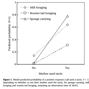

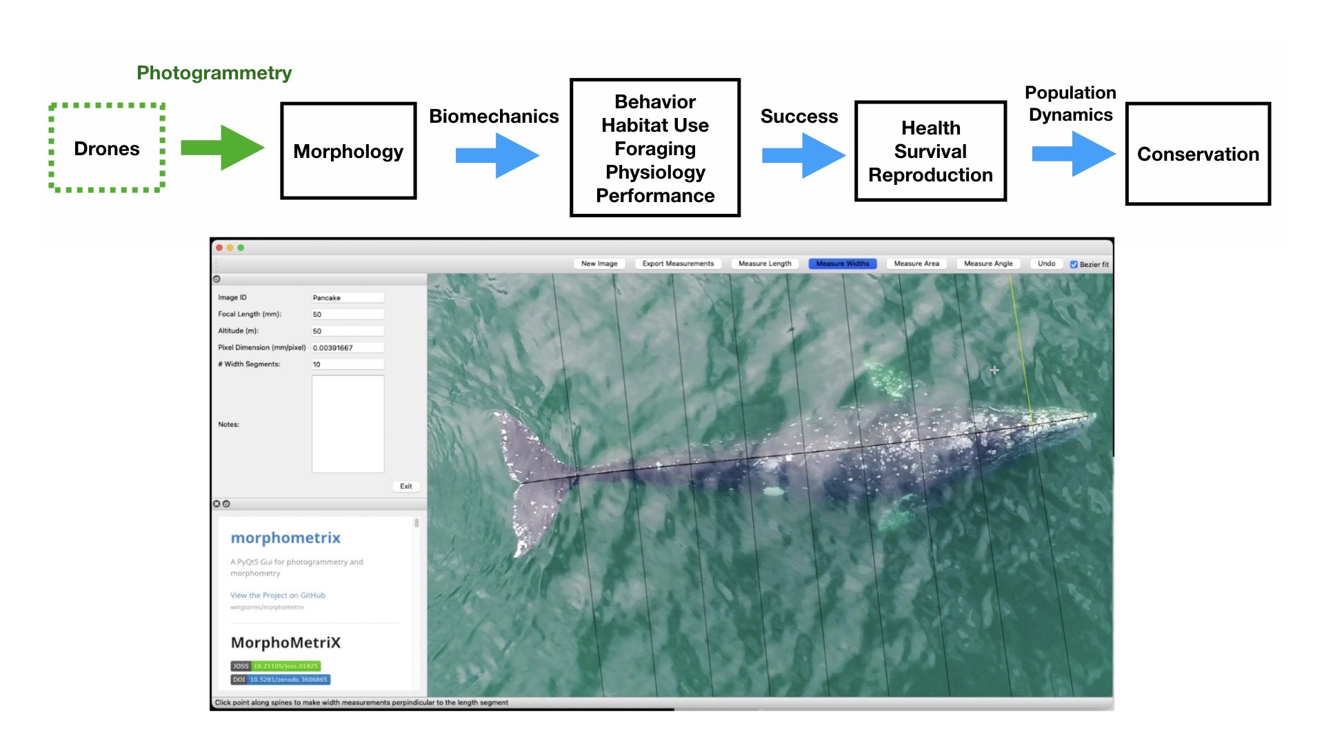
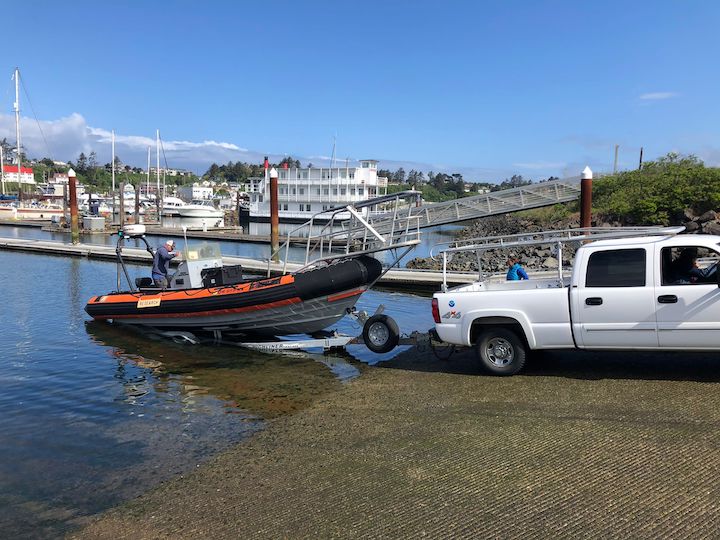


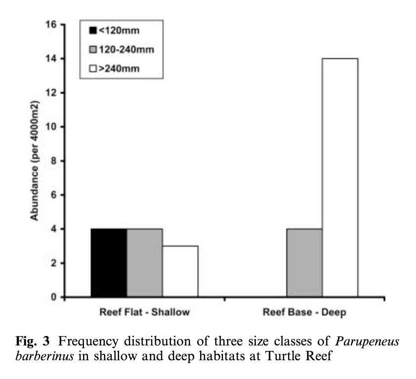
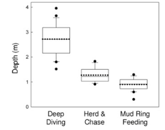


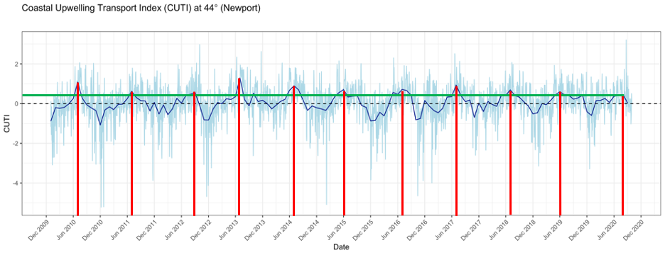