By Lisa Hildebrand, PhD student, OSU Department of Fisheries, Wildlife, & Conservation Sciences, Geospatial Ecology of Marine Megafauna Lab
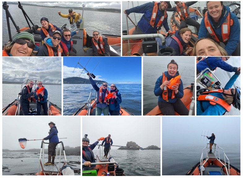
The winds are consistently (and sometimes aggressively) blowing from the north here on the Oregon coast, which can only mean one thing – summer has arrived! Since mid-May, the GRANITE (Gray whale Response to Ambient Noise Informed by Technology and Ecology) team has been looking for good weather windows to survey for gray whales and we have managed to get five great field work days already. In today’s blog post, I am going to share what (and who) we have seen so far.
On our first day of the field season, PI Leigh Torres, postdoc KC Bierlich and myself, were joined by a special guest: Dr. Andy Read. Andy is the director of the Duke University Marine Lab, where he also runs his own lab, which focuses on conservation biology and ecology of marine vertebrates. Andy was visiting the Hatfield Marine Science Center as part of the Lavern Weber Visiting Scientist program and was hosted here by Leigh. For those of you that do not know, Andy was Leigh’s graduate school advisor at Duke where she completed her Master’s and doctoral degrees. It felt very special to have Andy on board our RHIB Ruby for the day and to introduce him to some friends of ours. The first whale we encountered that day was “Pacman”. While we are always excited to re-sight an individual that we know, this sighting was especially mind-blowing given the fact that Leigh had “just” seen Pacman approximately two months earlier in Guerrero Negro, one of the gray whale breeding lagoons in Mexico (read this blog about Leigh and Clara’s pilot project there). Aside from Pacman, we saw five other individuals, all of which we had seen during last year’s field season.

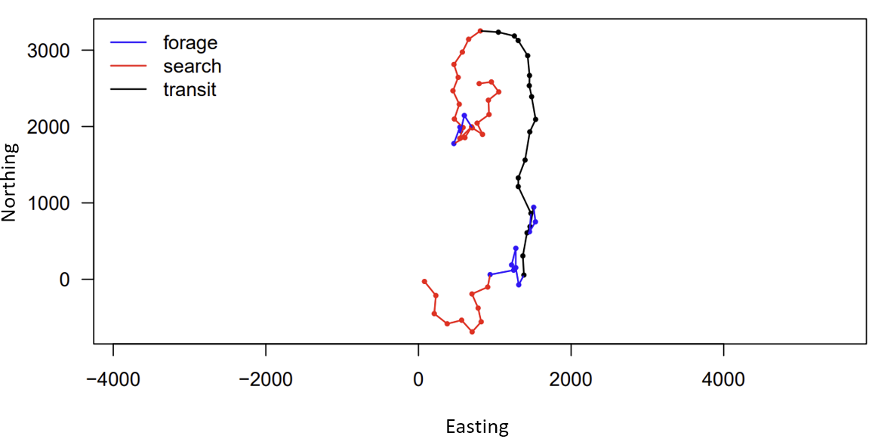
Since that first day on the water, we have conducted field work on four additional days and so far, we have only encountered known individuals in our catalog. This fact is exciting because it highlights the strong site fidelity that Pacific Coast Feeding Group (PCFG) gray whales have to areas within their feeding range. In fact, I am examining the residency and space use of each individual whale we have observed in our GRANITE study for one of my PhD chapters to better understand the level of fidelity individuals have to the central Oregon coast. Furthermore, this site fidelity underpins the unique, replicate data set on individual gray whale health and ecology that the GRANITE project has been able to progressively build over the years. So far during this field season in 2023, we have seen 13 unique individuals, flown the drone over 10 of them and collected four fecal samples from two, which represent critical data points from early on in the feeding season.
Our sightings this year have not only highlighted the high site fidelity of whales to our study area but have also demonstrated the potential for internal recruitment of calves born to “PCFG mothers” into the PCFG. Recruitment to a population can occur in two ways: externally (individuals immigrate into a population from another population) or internally (calves born to females that are part of the population return to, or stay, within their mothers’ population). Three of the whales we have seen so far this year are documented calves from females that are known to consistently use the PCFG range, including our central Oregon coast study area. In fact, we documented one of these calves, “Lunita”, just last year with her mother (see Clara’s recap of the 2022 field season blog for more about Lunita). The average calf survival estimate between 1997-2017 for the PCFG was 0.55 (Calambokidis et al. 2019), though it varied annually and widely (range: 0.34-0.94). Considering that there have been years with calf survival estimates as low as ~30%, it is therefore all the more exciting when we re-sight a documented calf, alive and well!

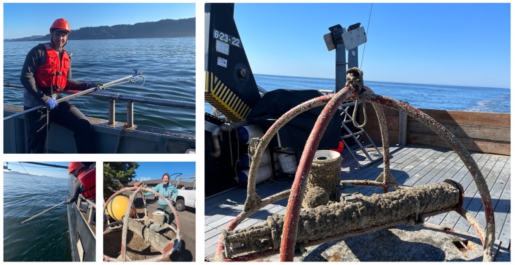
We have also been collecting data on the habitat and prey in our study system by deploying our paired GoPro/RBR sensor system. We use the GoPro to monitor the benthic substrate type and relative prey densities in areas where whales are feeding. The RBR sensor collects high-frequency, in-situ dissolved oxygen and temperature data, enabling us to relate environmental metrics to relative prey measurements. Furthermore, we also collect zooplankton samples with a net to assess prey community and quality. On our five field work days this year, we have predominantly collected mysid shrimp, including gravid (a.k.a. pregnant) individuals, however we have also caught some Dungeness and porcelain crab larvae. The GEMM Lab is also continuing our collaboration with Dr. Susanne Brander’s lab at OSU and her PhD student Lauren Kashiwabara, who plan on conducting microplastic lab experiments on wild-caught mysid shrimp. Their plan is to investigate the growth rates of mysid shrimp under different temperature, dissolved oxygen, and microplastic load conditions. However, before they can begin their experiments, they need to successfully culture the mysids in the lab, which is why we collect samples for them to use as their ‘starter culture’. Stay tuned to hear more about this project as it develops!
So, all in all, it has been an incredibly successful start to our field season, marked by the return of many familiar flukes and flanks! We are excited to continue collecting rock solid GRANITE data this summer to increase our efforts to understand gray whale ecology and physiology.
References
Calambokidis, J., Laake, J., and Perez, A. (2019). Updated analyses of abundance and population structure of seasonal gray whales in the Pacific Northwest, 1996-2017. IWC, SC/A17/GW/05 for the Workshop on the Status of North Pacific Gray Whales. La Jolla: IWC.