By Lisa Hildebrand, PhD candidate, OSU Department of Fisheries, Wildlife, & Conservation Sciences, Geospatial Ecology of Marine Megafauna Lab
Baleen whales must navigate a seemingly featureless world to locate the resources they need to survive. The task of finding prey to feed on in the vast seascapes relies on the use of several sensory modalities that operate at different scales (Torres 2017; Figure 1). For example, baleen whale vision is believed to be rather limited, with the ability to see objects about 10-100 meters away. Yet, baleen whale somatosensory perception of oceanographic stimuli is thought to be on the order of 100-1000s kilometers. This diversity in sensory ability has led scientists to believe that whales, in fact all animals, perceive cues and make decisions at several scales. As ecologists, we endeavor to understand why and when animals are found (or not found) in certain locations as this knowledge allows us to better manage and conserve animal populations. With this information we can aim to minimize potential anthropogenic disturbance and protect important resource areas, such as foraging or nursing grounds. In order to accomplish this goal, we ourselves must conduct studies and test hypotheses at several scales (Levin 1992; Hobbs 2003). As someone who tackles spatial foraging ecology questions, I am particularly interested in understanding whale behavior and movement in the context of feeding. Since accurately measuring predator and prey distribution at the same scales can be challenging, we often resort to environmental variables to serve as proxies for prey, whereby we look for correlations between environmental variables and whales to understand and predict the distribution of our population.

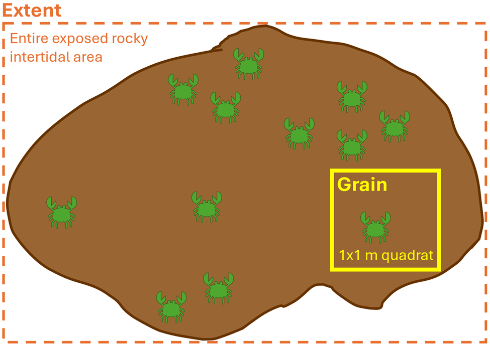
What do I mean when I use the word ‘scale’? The term scale is typically explained by two components: grain and extent (Wiens 1989). The grain is the finest resolution measured; in other words, how detailed we are measuring. The extent is the overall coverage of what we are measuring. These components can be applied to both spatial scale and temporal scale. For example, spatially, if we were using a 1×1 meter sampling quadrat to count the number of crabs on a rocky shore, then our grain would be the 1 m2 quadrat and the extent would be the entire exposed rocky intertidal area that we are surveying (Figure 2). Temporally, if we placed a temperature logger at the mouth of Yaquina Bay that took a temperature recording every minute for two years, then our grain would be one minute and the extent would be two years. So, when designing a study, it is imperative for us to decide on the spatiotemporal scales of the ecological questions we are asking and the hypotheses we are testing, as it will inform what data we need to collect. When making this decision, it is important to think about the scale at which the ecological process happens, as opposed to the scale at which we can observe the process (Levin 1992). In other words, we need to think from the perspective of our study species, as opposed to from our own human perspective. Making informed and ecologically reasonable decisions regarding the choice of scale relies on having prior knowledge of an animal’s biology, such as knowing that baleen whales might see a prey patch that is 50 meters away, but it may also somatosensorily perceive an oceanic front where zooplankton prey aggregate from 500 kilometers away.
There is a wealth of studies that have explored space use patterns of wildlife relative to environmental variables to better understand foraging behavior. I want to share a couple from the marine mammal realm with you that I find particularly fascinating. In their 2018 study, González García and colleagues used opportunistic sightings of blue whales around the Azorean islands of Portugal and modeled their distribution patterns relative to physiographic and oceanographic variables summarized at different spatial (fine [1-10 km] and meso [10-100 km]) and temporal (daily, weekly, monthly) scales. The two variables that were most correlated with blue whale occurrence was distance from the coast and eddy kinetic energy (a measure of mesoscale variability of ocean dynamics). Both of these variables were interestingly found to be scale invariant, meaning that no matter which spatial and temporal scale was investigated, the relationship between blue whales and these two variables stayed the same; blue whale occurrence increased with increasing distance from the coast and was maximal at an eddy kinetic energy value of 0.007 cm2/s2 (Figure 3).

However, not all studies find scale invariant relationships. For example, Cotté and co-authors (2009) found that habitat use of Mediterranean fin whales was very much scale dependent. At a large scale (700-1,000 km and annual), fin whales were more densely aggregated during the summer in the Western Mediterranean where there was consistently colder water than in the winter. However, at a meso scale (20-100 km and weekly-monthly), fin whale densities were highest in areas where there were steep changes in temperature, as opposed to consistently cold temperatures. The authors explain that these differences in fin whale density and temperature at different scales are likely due to whale movement being driven by annually persistent prey abundance at the large scale, but at the meso scale, where prey aggregations are less predictable, the fin whales’ distribution becomes more driven by areas of physical ocean mixing.
As I investigate the environmental drivers of individual gray whale space use using our 8-year GRANITE (Gray whale Response to Ambient Noise Informed by Technology and Ecology) dataset, these studies (and many more) are at the top of my mind to interpret the patterns we are detecting. Our goal is to quantify and describe what environmental conditions (1) lead to a higher probability of a gray whale being seen in our central Oregon coast study area (~70 km) at a daily scale, and (2) influence space use patterns (activity range, residency, activity center) of different individual whales at annual scales. Our results show both consistency and variation in the environmental drivers of gray whales across these scales, leading me to deeply consider how gray whales make decisions at different points in their lives, based on information gained through various senses, to maximize their chances of capturing food. Previous work from the GEMM Lab on the relationships between gray whales and prey, at both fine (read more here) and large (read more here) scales have guided my work by providing specific hypotheses regarding environmental variables and lag times for me to test. Investigating the environmental drivers of animal space use and behavior is exciting work as it reveals that no single environmental variable determines animal distribution, but rather that multiple processes are happening concomitantly that animals respond to at different scales continually. It is only by studying animal space use patterns across spatiotemporal scales that we can begin to understand their complex decision-making patterns.
Did you enjoy this blog? Want to learn more about marine life, research, and conservation? Subscribe to our blog below and get a monthly message when we post a new blog. Just add your name and email into the subscribe box below.
References
Cotté, C., Guinet, C., Taupier-Letage, I., Mate, B., & Petiau, E. (2009). Scale-dependent habitat use by a large free-ranging predator, the Mediterranean fin whale. Deep Sea Research Part I: Oceanographic Research Papers, 56(5), 801-811.
González García, L., Pierce, G. J., Autret, E., & Torres-Palenzuela, J. M. (2018). Multi-scale habitat preference analyses for Azorean blue whales. PLoS One, 13(9), e0201786.
Hobbs, N. T. (2003). Challenges and opportunities in integrating ecological knowledge across scales. Forest Ecology and Management, 181(1-2), 223-238.
Levin, S. A. (1992). The problem of pattern and scale in ecology: the Robert H. MacArthur award lecture. Ecology, 73(6), 1943-1967.
Torres, L. G. (2017). A sense of scale: Foraging cetaceans’ use of scale‐dependent multimodal sensory systems. Marine Mammal Science, 33(4), 1170-1193.
Wiens, J. A. (1989). Spatial scaling in ecology. Functional ecology, 3(4), 385-397.