Hello from Palmer Station, Antarctica! I’ve spent the last five months here in a kind of parallel universe to that of my normal life in Oregon. It’s spring here at the Western Antarctic Peninsula (WAP), and since May I’ve been part of a team studying Antarctic krill (Euphausia superba) – a big change from the Oregon species I typically study, and one that has already taught me so much.
I am here as part of a project titled “The Omnivore’s Dilemma: The effect of autumn diet on winter physiology and condition of juvenile Antarctic krill”. Through at-sea fieldwork and experiments in the lab, we have spent this field season investigating how climate-driven changes in diet impact juvenile and adult krill health during the long polar night. Winter is a crucial time for krill survival and recruitment, and an understudied season in this remote corner of the world.
Within this field season, we have been part of two great research cruises along the WAP, and spent the rest of the time at Palmer Station, running long-term experiments to learn how diet influences krill winter growth and development. The time has passed incredibly fast, and it’s hard to believe that we’ll be heading home in just a couple weeks.
There have been so many wonderful parts to our time here. While at sea, I was constantly aware that each new bay and fjord we sampled was one of the most beautiful places I would ever have the privilege to visit. I was also surprised and thrilled by the number of whales we saw – I recorded over one hundred sightings, including humpbacks, minke, and killer whales. As consumed as I was by looking for whales during the few hours of daylight, it was also rewarding to broaden my marine mammal focus and learn about another krill predator, the crabeater seal, from a great team researching their ecology and physiology.
In between our other work, I have been processing active acoustic (echosounder) data collected during a winter 2022 cruise that visited many of the same regions of the WAP. Antarctic krill have been much more thoroughly studied than the main krill species that occur off the coast of Oregon, Euphausia pacifica and Thysanoessa spinifera, and it has been amazing to draw upon this large body of literature.
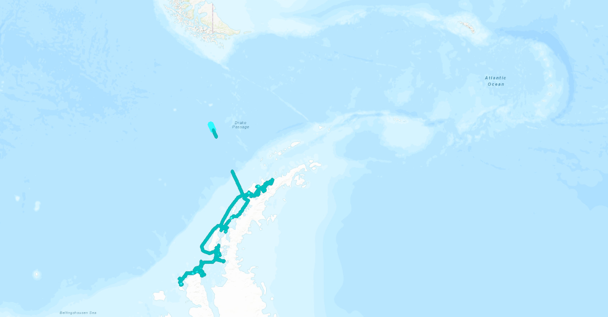
Figure 2. The active acoustic data I’m working with from the Western Antarctic Peninsula, pictured here, was collected along a wiggly cruise track in 2022, giving me the opportunity to learn how to process this type of survey data and appreciate the ways in which a ship’s movements translate to data analysis.
Working with a new flavor of echosounder data has presented me with puzzles that are teaching me to navigate different modes of data collection and their analytical implications, such as for the cruise track data above. I’ll never take data collected along a standardized grid for granted again!
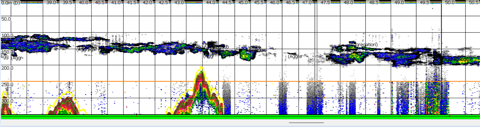
I’ve also learned new techniques that I am excited to apply to my research in the Northern California Current (NCC) region. For example, there are two primary different ways of detecting krill swarms in echosounder data: by comparing the results of two different acoustic frequencies, and by training a computer algorithm to recognize swarms based on their dimensions and other characteristics. After trying a few different approaches with the Antarctic data this season, I developed a way to combine these techniques. In the resulting dataset, two different methods have confirmed that a given area represents krill, which gives me a lot of confidence in it. I’m looking forward to applying this technique to my NCC data, and using it to assess some of my next research questions.
Figure 3. A combination of krill detection techniques selected these long krill aggregations off the coast of the Western Antarctic Peninsula (WAP).
Throughout it all, the highlight of this season has been being part of an amazing field team. I’m here with Kim Bernard (as a co-advised student, I refer to Kim as my “krill advisor” and Leigh as my “whale advisor”), and undergraduate Abby Tomita, who just started her senior year at OSU remotely from Palmer. From nights full of net tows to busy days in the lab, we’ve become a well-oiled machine, and laughed a lot along the way. Working with the two of them makes me sure that we’ll be able to best any difficulties that come up.
Now, our next challenge is wrapping up our last labwork, packing up equipment and samples, and getting ready to say goodbye. Leaving this wild, remote place is always heartbreaking – you never really know if you’ll be back. But there’s a lot to look forward to as we journey north, too: I can’t wait to hug my family and friends, eat a salad, and drive out to Newport to see the GEMM Lab. I’m excited to head back to the world with everything I’ve learned here, and to keep working.
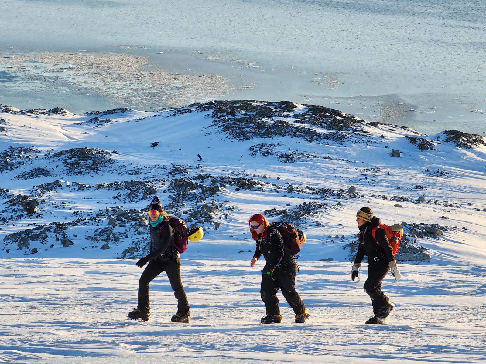
Figure 4. Kim (left), Abby (middle), and I (right) hike on the Marr Ice Piedmont during a gorgeous day off.
By Rachel Kaplan, PhD student, OSU College of Earth, Ocean and Atmospheric Sciences and Department of Fisheries, Wildlife, & Conservation Sciences, Geospatial Ecology of Marine Megafauna Lab
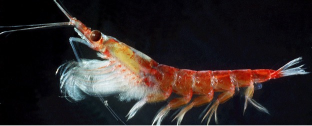
Krill, a shrimplike crustacean found across our oceans, embodies the term “small but mighty”. Though individuals tend to be small, sometimes weighing in at less than a gram, the numerous species of krill have a global distribution and are estimated to collectively outweigh the entire human population. Much of my graduate research focuses on relationships between foraging whales and krill (Euphausia pacifica and Thysanoessa spinifera) in the Northern California Current (NCC) region. This work hinges on themes that are universal across environments: just as krill are ubiquitous across the global ocean, questions of prey quality, distribution, and ecological relationships with predators are universal.
Next week, I’m headed south to consider these questions in a very different foraging environment: the Western Antarctic Peninsula (WAP). One benefit of being a co-advised student is the incredible opportunity to be exposed to diverse projects and types of research. My graduate co-advisor, Kim Bernard, has studied krill in the WAP region for over a decade, and she is currently leading research into the implications of the shifting polar food web for Antarctic krill (Euphasia superba). Through a series of laboratory experiments and fieldwork, the project, titled “The Omnivore’s Dilemma: The effect of autumn diet on winter physiology and condition of juvenile Antarctic krill”, investigates the impact of climate-driven changes in diet on the health of juvenile krill in autumn and winter, a key time for their survival and recruitment. Winter is a poorly studied season in Antarctica, and this project has already shed light on the physiology, respiration, and growth potential of juvenile krill (Bernard et al., 2022).
Figure 1: Antarctic krill are much bigger than those found in the NCC region – they can be as long as your thumb! (Source: Australian Antarctic Program)
Just as in the NCC region, krill are an essential link in Southern Ocean food webs, where they transfer energy from their microscopic prey to the higher trophic levels that eat them, including several species of fish, seals, penguins, and whales (Bernard & Steinberg, 2013; Cavan et al., 2019; Ducklow et al., 2013). These predators depend upon this high-quality prey to fuel their seasonal migrations and to build the energy reserves they need to survive the frigid Antarctic winter (Cade et al., 2022; Schaafsma et al., 2018). But, the quality of krill depends upon the food that it can consume itself, and climate change may alter their diet.
There’s a lot to love about krill, but my fascination with them is directly tied to their value as a food source for predators. I want to know how the caloric content of individuals and the aggregations they form changes spatially along the WAP, and how this might shift under climate-forced food web changes. This work will clarify the climate-driven variability in the quality of krill as prey, and the implications this might have for top predators in the region.
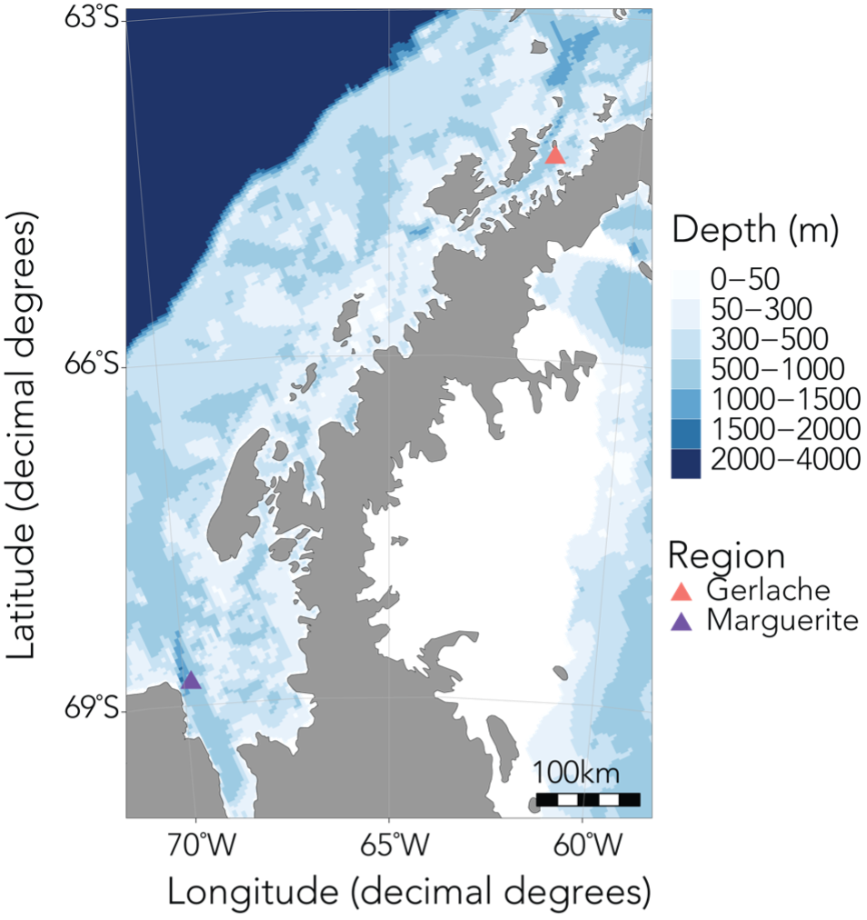
Figure 2: The upcoming field season will involve sampling krill along a latitudinal gradient in the WAP region, spanning approximately from the Gerlache Strait in the north to Marguerite Bay in the south (Bernard et al., 2022).
In order to investigate these questions, I’ll be spending the next six months based out of Palmer Station, the smallest of the United States’ research bases in Antarctica, along with Kim and our undergraduate intern Abby. During this upcoming field season, we’ll spend about a month at sea collecting krill samples and active acoustic data using an echosounder, and the rest of the time conducting experiments and sampling in the nearshore. Over the last year, Abby has worked with me to quantify krill caloric content in the NCC, as well as processing samples collected in Antarctica last year. I’m so impressed by everything she’s accomplished, and excited to see her take in this environment, learn a fresh set of experimental and field sampling approaches, and be inspired to ask new questions.
For me, heading south will be a bit like coming home. After graduating from college, I spent about nine months living at Palmer Station and working on the microbial ecology component of the long-term ecological research station there. The experience of being immersed in the WAP environment was foundational to my curiosity about ocean ecology and the impacts of climate change. It is also where I met Kim! All in all, this environment fueled my desire to study krill with Kim and spatial ecology with Leigh, and set me on the course I’m on today.
It also feels meaningful to return here again at this point in my educational journey. With new knowledge and questions I have formed while working in the NCC, I am now excited to apply this knowledge and consider similar questions in the WAP. Abby and I will write blogs through the season and post them here, so stay tuned for news from down south!
Figure 4: Kim and I (the two farthest right in the front row) prepare for a group costumed polar plunge in 2015. Will we do it again? We’ll keep you posted!
References
Bernard, K. S., & Steinberg, D. K. (2013). Krill biomass and aggregation structure in relation to tidal cycle in a penguin foraging region off the Western Antarctic Peninsula. ICES Journal of Marine Science, 70(4), 834–849. https://doi.org/10.1093/icesjms/fst088
Bernard, K. S., Steinke, K. B., & Fontana, J. M. (2022). Winter condition, physiology, and growth potential of juvenile Antarctic krill. Frontiers in Marine Science, 9, 990853. https://doi.org/10.3389/fmars.2022.990853
Cade, D. E., Kahane-Rapport, S. R., Wallis, B., Goldbogen, J. A., & Friedlaender, A. S. (2022). Evidence for Size-Selective Predation by Antarctic Humpback Whales. Frontiers in Marine Science, 9, 747788. https://doi.org/10.3389/fmars.2022.747788
Cavan, E. L., Belcher, A., Atkinson, A., Hill, S. L., Kawaguchi, S., McCormack, S., Meyer, B., Nicol, S., Ratnarajah, L., Schmidt, K., Steinberg, D. K., Tarling, G. A., & Boyd, P. W. (2019). The importance of Antarctic krill in biogeochemical cycles. Nat Commun, 10(1), 4742. https://doi.org/10.1038/s41467-019-12668-7
Ducklow, H., Fraser, W., Meredith, M., Stammerjohn, S., Doney, S., Martinson, D., Sailley, S., Schofield, O., Steinberg, D., Venables, H., & Amsler, C. (2013). West Antarctic Peninsula: An Ice-Dependent Coastal Marine Ecosystem in Transition. Oceanography, 26(3), 190–203. https://doi.org/10.5670/oceanog.2013.62
Schaafsma, F. L., Cherel, Y., Flores, H., van Franeker, J. A., Lea, M.-A., Raymond, B., & van de Putte, A. P. (2018). Review: The energetic value of zooplankton and nekton species of the Southern Ocean. Marine Biology, 165(8), 129. https://doi.org/10.1007/s00227-018-3386-z
Allison Dawn, new GEMM Lab Master’s student, OSU Department of Fisheries, Wildlife and Conservation Sciences, Geospatial Ecology of Marine Megafauna Lab
While standing at the Stone Shelter at the Saint Perpetua Overlook in 2016, I took in the beauty of one of the many scenic gems along the Pacific Coast Highway. Despite being an East Coast native, I felt an unmistakable draw to Oregon. Everything I saw during that morning’s hike, from the misty fog that enshrouded evergreens and the ocean with mystery, to the giant banana slugs, felt at once foreign and a place I could call home. Out of all the places I visited along that Pacific Coast road trip, Oregon left the biggest impression on me.
Figure 1. View from the Stone Shelter at the Cape Perpetua Overlook, Yachats, OR. June 2016.
For my undergraduate thesis, which I recently defended in May 2021, I researched blue whale surface interval behavior. Surface interval events for oxygen replenishment and rest are a vital part of baleen whale feeding ecology, as it provides a recovery period before they perform their next foraging dive (Hazen et al., 2015; Roos et al., 2016). Despite spending so much time studying the importance of resting periods for mammals, that 2016 road trip was my last true extended resting period/vacation until, several years later in 2021, I took another road trip. This time it was across the country to move to the place that had enraptured me.
Now that I am settled in Corvallis, I have reflected on my journey to grad school and my recent road trip; both prepared me for a challenging and exciting new chapter as an incoming MSc student within the Marine Mammal Institute (MMI).
Part 1: Journey to Grad School
When I took that photo at the Cape Perpetua Overlook in 2016, I had just finished the first two semesters of my undergraduate degree at UNC Chapel Hill. As a first-generation, non-traditional student those were intense semesters as I made the transition from a working professional to full-time undergrad.
By the end of my freshman year I was debating exactly what to declare as my major, when one of my marine science TA’s, Colleen, (who is now Dr. Bove!), advised that I “collect experiences, not degrees.” I wrote this advice down in my day planner and have never forgotten it. Of course, obtaining a degree is important, but it is the experiences you have that help lead you in the right direction.
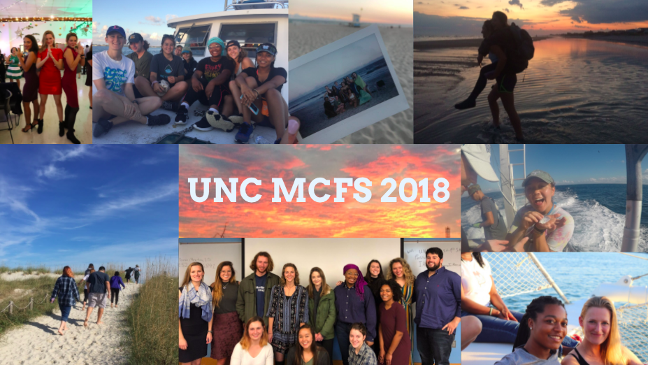
That advice was one of the many reasons I decided to participate in the Morehead City Field Site program, where UNC undergraduates spend a semester at the coast, living on the Duke Marine Lab’s campus in Beaufort, NC. During that semester, students take classes to fulfill a marine science minor while participating in hands-on research, including an honors thesis project. The experience of designing, carrying out, and defending my own project affirmed that graduate school in the marine sciences was right for me. As I move into my first graduate TA position this fall, I hope to pay forward that encouragement to other undergraduates who are making decisions about their own future path.
Figure 2. Final slide from my honors thesis defense. UNC undergraduates, and now fellow alumni, who participated in the Morehead City Field Site program in Fall 2018.
Part 2: Taking a Breather
Like the GEMM Lab’s other new master’s student Miranda, my road trip covered approximately 2,900 miles. I was solo for much of the drive, which meant there was no one to argue when I decided to binge listen to podcasts. My new favorite is How To Save A Planet, hosted by marine biologist Dr. Ayana Elizabeth Johnson and Alex Blumberg. At the end of each episode they provide a call to action & resources for listeners – I highly recommend this show to anyone interested in what you can do right now about climate change.
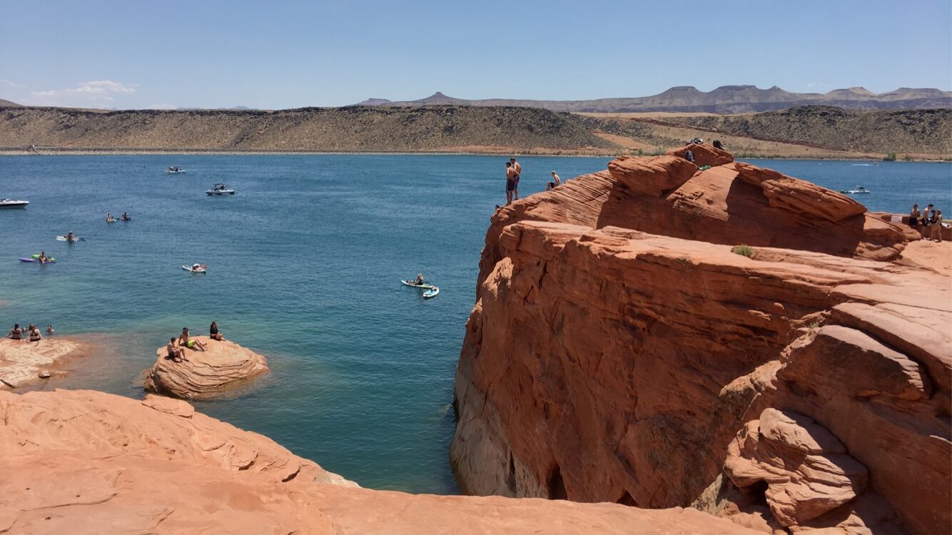
Along my trip I took a stop in Utah to visit my parents. I had never been to a desert basin before and engaged in many desert-related activities: visiting Zion National Park, hiking in 116-degree heat, and facing my fear of heights via cliff jumping.
Figure 3. Sandstone Rocks at Sand Hollow National Park, Hurricane, Utah. June 2021.
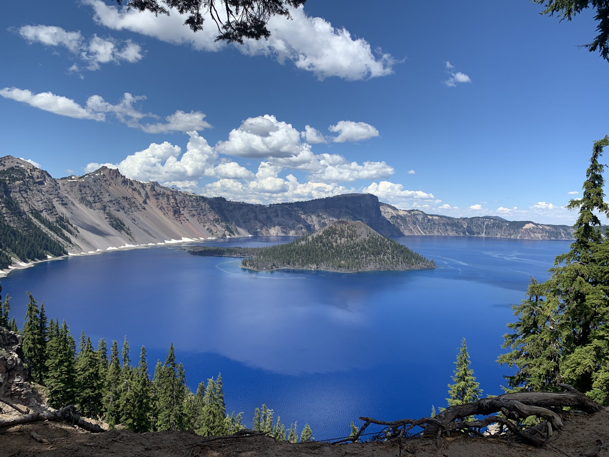
My parents wanted to help me settle into my new home, as parents do, so we drove the rest of the way to Oregon together. As this would be their first visit to the state, we strategically planned a trip to Crater Lake as our final scenic stop before heading into Corvallis.
Figure 4. Wizard Island in Crater Lake National Park, Klamath County, OR. June 2021.
This time off was filled with adventure, yet was restorative, and reminded me the importance of taking a break. I feel ready and refreshed for an intense summer of field work.
Part 3: Rested and Ready
Despite accumulating skills to do research in the field over the years, I have yet to do marine mammal field work (or even see a whale in person for that matter.) My mammal research experience included analyzing drone imagery, behind a computer, that had already been captured. As you can imagine, I am extremely excited to join the Port Orford team as part of the TOPAZ/JASPER projects this summer, collecting ecological data on gray whales and their prey. I will be learning the ropes from Lisa Hildebrand and soaking up as much information as possible as I will be taking over as lead for this project next year.
It will take some time before my master’s thesis is fully developed, but it will likely focus on assessing the environmental factors that influence gray whale zooplankton prey availability, and the subsequent impacts on whale movements and health. For five years, the Port Orford project has conducted GoPro drops at 12 sampling stations to collect data on zooplankton relative abundance.
Figures 5 & 6. GEMM GoPro drop stick assembly and footage demonstrating mysid data collection. July 2021.
Paired with this GoPro is a Time-Depth Recorder (TDR) that provides temperature and depth data. The 2021 addition to this GoPro system is a new dissolved oxygen (DO) sensor the GEMM Lab has just acquired. This new piece of equipment will add to the set of parameters we can analyze to describe what and how oceanographic factors drive prey variability and gray whale presence in our study site.My first task as a GEMM Lab student is to get to know this DO sensor, figure out how it works, set it up, test it, attach it to the GoPro device, and prepare it for data collection during the upcoming Port Orford project starting in 1 week!
Figure 7. The GEMM lab’s new RBR solo3 getting ready for Port Orford. July 2021.
Dissolved oxygen plays a vital role in the ocean; however, climate change and increased nutrient loading has caused the ocean to undergo deoxygenation. According to the IUCN’s 2019 Issues Brief, these factors have resulted in an oxygen decline of 2% since the middle of the 20th century, with most of this loss occurring within the first 1000 meters of the ocean. Two percent may not seem like much, but many species have a narrow oxygen threshold and, like pH changes in coral reef systems, even slight changes in DO can have an impact. Additionally, the first 1000 meters of the ocean contains the greatest amount of species richness and biodiversity.
Previous research done in a variety of systems (i.e., estuarine, marine, and freshwater lakes) shows that dissolved oxygen concentrations can have an impact on predator-prey interactions, where low dissolved oxygen results in decreased predation (Abrahams et al., 2007; Breitburg et al., 1997; Domenici et al., 2007; Kramer et al., 1987); and changes in DO also change prey vertical distributions (Decker et al., 2004). In Port Orford, we are interested in understanding the interplay of factors driving zooplankton community distribution and abundance while investigating the trophic interaction between gray whales and their prey.
I have spent some time with our new DO sensor and am looking forward to its first deployments in Port Orford! Stay tuned for updates from the field!
References
Abrahams, M. V., Mangel, M., & Hedges, K. (2007). Predator–prey interactions and changing environments: who benefits?. Philosophical Transactions of the Royal Society B: Biological Sciences, 362(1487), 2095-2104.
Breitburg, D. L., Loher, T., Pacey, C. A., & Gerstein, A. (1997). Varying effects of low dissolved oxygen on trophic interactions in an estuarine food web. Ecological Monographs, 67(4), 489-507.
Decker, M. B., Breitburg, D. L., & Purcell, J. E. (2004). Effects of low dissolved oxygen on zooplankton predation by the ctenophore Mnemiopsis leidyi. Marine Ecology Progress Series, 280, 163-172.
Domenici, P., Claireaux, G., & McKenzie, D. J. (2007). Environmental constraints upon locomotion and predator–prey interactions in aquatic organisms: an introduction.
Hazen, E. L., Friedlaender, A. S., & Goldbogen, J. A. (2015). Blue whales (Balaenoptera musculus) optimize foraging efficiency by balancing oxygen use and energy gain as a function of prey density. Science Advances, 1(9), e1500469.
Kramer, D. L. (1987). Dissolved oxygen and fish behavior. Environmental biology of fishes, 18(2), 81-92.
Roos, M. M., Wu, G. M., & Miller, P. J. (2016). The significance of respiration timing in the energetics estimates of free-ranging killer whales (Orcinus orca). Journal of Experimental Biology, 219(13), 2066-2077.
Clara Bird, PhD Student, OSU Department of Fisheries, Wildlife, and Conservation Sciences, Geospatial Ecology of Marine Megafauna Lab
When I thought about what doing fieldwork would be like, before having done it myself, I imagined that it would be a challenging, but rewarding and fun experience (which it is). However, I underestimated both ends of the spectrum. I simultaneously did not expect just how hard it would be and could not imagine the thrill of working so close to whales in a beautiful place. One part that I really did not consider was the pre-season phase. Before we actually get out on the boats, we spend months preparing for the work. This prep work involves buying gear, revising and developing protocols, hiring new people, equipment maintenance and testing, and training new skills. Regardless of how many successful seasons came before a project, there are always new tasks and challenges in the preparation phase.
For example, as the GEMM Lab GRANITE project team geared up for its seventh field season, we had a few new components to prepare for. Just to remind you, the GRANITE (Gray whale Response to Ambient Noise Informed by Technology and Ecology) project’s field season typically takes place from June to mid-October of each year. Throughout this time period the field team goes out on a small RHIB (rigid hull inflatable boat), whenever the weather is good enough, to collect photo-ID data, fecal samples, and drone imagery of the Pacific Coast Feeding Group (PCFG) gray whales foraging near Newport, OR, USA. We use the data to assess the health, ecology and population dynamics of these whales, with our ultimate goal being to understand the effect of ambient noise on the population. As previous blogs have described, a typical field day involves long hours on the water looking for whales and collecting data. This year, one of our exciting new updates is that we are going out on two boats for the first part of the field season and starting our season 10 days early (our first day was May 20th). These updates are happening because a National Science Foundation funded seismic survey is being conducted within our study area starting in June. The aim of this survey is to assess geophysical structures but provides us with an opportunity to assess the effect of seismic noise on our study group by collecting data before, during, and after the survey. So, we started our season early in order to capture the “before seismic survey” data and we are using a two-boat approach to maximize our data collection ability.
While this is a cool opportunistic project, implementing the two-boat approach came with a new set of challenges. We had to find a second boat to use, buy a new set of gear for the second boat, figure out the best way to set up our gear on a boat we had not used before, and update our data processing protocols to include data collected from two boats on the same day. Using two boats also means that everyone on the core field team works every day. This core team includes Leigh (lab director/fearless leader), Todd (research assistant), Lisa (PhD student), Ale (new post-doc), and me (Clara, PhD student). Leigh and Todd are our experts in boat driving and working with whales, Todd is our experienced drone pilot, I am our newly certified drone pilot, and Lisa, Ale, and myself are boat drivers. Something I am particularly excited about this season is that Lisa, Ale, and I all have at least one field season under our belts, which means that we get to become more involved in the process. We are learning how to trailer and drive the boats, fly the drones, and handling more of the post-field work data processing. We are becoming more involved in every step of a field day from start to finish, and while it means taking on more responsibility, it feels really exciting. Throughout most of graduate school, we grow as researchers as we develop our analytical and writing skills. But it’s just as valuable to build our skillset for field work. The ocean conditions were not ideal on the first day of the field season, so we spent our first day practicing our field skills.
For our “dry run” of a field day, we went through the process of a typical day, which mostly involved a lot of learning from Leigh and Todd. Lisa practiced her trailering and launching of the boat (figure 1), Ale and Lisa practiced driving the boat, and I practiced flying the drone (figure 2). Even though we never left the bay or saw any whales, I thoroughly enjoyed our dry run. It was useful to run through our routine, without rushing, to get all the kinks out, and it also felt wonderful to be learning in a supportive environment. Practicing new skills is stressful to say the least, especially when there is expensive equipment involved, and no one wants to mess up when they’re being watched. But our group was full of support and appreciation for the challenges of learning. We cheered for successful boat launchings and dockings, and drone landings. I left that day feeling good about practicing and improving my drone piloting skills, full of gratitude for our team and excited for the season ahead.
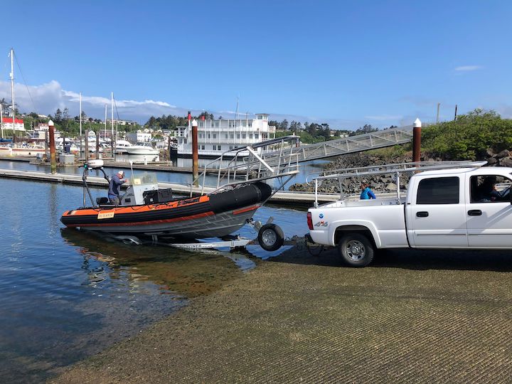
Figure 1. Lisa (driving the truck) launching the boat.
Figure 2. Clara (seated, wearing a black jacket) landing the drone in Ale’s hands.
All the diligent prep work paid off on Saturday with a great first day (figure 3). We conducted five GoPro drops (figure 4), collected seven fecal samples from four different whales (figure 5), and flew four drone flights over three individuals including our star from last season, Sole. Combined, we collected two trifectas (photo-ID images, fecal samples, and drone footage)! Our goal is to get as many trifectas as possible because we use them to study the relationship between the drone data (body condition and behavior) and the fecal sample data (hormones). We were all exhausted after 10 hours on the water, but we were all very excited to kick-start our field season with a great day.
Figure 3. Lisa on the bow pulpit during our first sighting of the day.
Figure 4. Lisa doing a GoPro drop, she’s lowering the GoPro into the water using the line in her hands.
Figure 5. Clara and Ale collecting a fecal sample.
On Sunday, just one boat went out to collect more data from Sole after a rainy morning and I successfully flew over her from launching to landing! We have a long season ahead, but I am excited to learn and see what data we collect. Stay tuned for more updates from team GRANITE as our season progresses!
Having worked almost exclusively on humpback whales for the past 5 years, I recently realized how specialized I have become when I was asked to participate in an expedition targeting another legendary cetacean, which I discovered I knew so little about: the sperm whale. On November 18th I boarded a catamaran with a team of 8 other seamen, film makers and scientists, all ready to sail off the west coast of New Caledonia in the search of this elusive animal. The expedition was named “Code CODA” in reference to the unique patterned series of clicks produced by sperm whales.
As I prepared for the expedition, I did my scientific literature homework and felt a growing awe for sperm whales. At every step of my research, whether I investigated their morphology, physiology, social behavior, feeding habits… everything about them appeared to be exceptional. Below is a list summarizing five mind-blowing facts everyone should know about sperm whales.
A sperm whale sketch I made on the boat in preparation for this blog post (Illustration credit: Solène Derville)
Sea giants
Sperm whales are the largest of the odontocetes species, which is the group of “toothed whales” that also includes dolphins, porpoises and beaked whales. They show a strong sexual dimorphism, unusual for a cetacean, as adult males can be about twice as big as adult females. Indeed, male sperm whales can reach up to 18 m and 56 tons (approximately the weight of 9 elephants!). Their massive block-shaped head is perhaps their most distinctive feature. It contains the largest brain in the animal kingdom and as a comparison, it is claimed that an entire car could fit in it! By its morphology alone, the sperm whale hence appears like an all-round champion of cetaceans.
Abyssal divers
Sperm whales are some of the best divers among air-breathing sea creatures. They have been recorded down to 2,250 m, and sperm whale carcasses have been found entangled in deep-sea cables suggesting that they can dive even deeper. In these dark and cold waters, sperm whales hunt for fish and squids (and sometimes check out ROVs, see videos of a surprising deep sea encounter made in 2015 off the coast of Louisiana, on Nautilus Live). They are renowned for attacking giant (Architeuthis spp) and colossal (Mesonychoteuthis hamiltoni) squids, which can reach more than 10 m in length. The squid sucker scars born by sperm whales give evidence of these titan combats. Because sperm whales only have teeth on the lower jaw, they cannot chew and may end up eating their prey alive. But every problem has its solution… sperm whales have evolved the longest digestive system in the world: it can reach 300 m long! Their stomach is divided into four compartments, the first of which is covered by a thick and muscular lining that can resist the assault of live prey.
Deluxe poopers
The digestion of sperm whale prey happens in the next digestive compartments, but one component will resist: the squids’ beaks! As beaks accumulate in the digestive system (up to 18,000 beaks were found in a specimen!), they cause an irritation that is responsible for the production of a waxy substance known as ‘ambergris’. After a while, this substance is thought to be occasionally secreted along with the whale’s poop (although it has been speculated that large pieces of ambergris might be expelled by the mouth… charming!). Ambergris may be found floating at sea or washed up on coastlines, where it may make one happy beachcomber! The latest report of such a lucky finding of ambergris in 2016 was estimated at more than US$71,000 for a 1.57 kg lump. Indeed, ambergris is a valued additive used in perfume, although it has now mostly been replaced by synthetic equivalents. The use of ambergris in cooking, incense or medication in ancient Egypt and the Middle Ages is also reported.
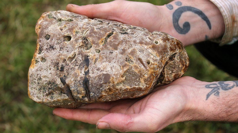
Ambergris lump found in the UK in 2018 (photo credit: APEX, source: https://www.bbc.com/news/uk-england-devon-42703991)
Caring whales
Sperm whales are highly social animals. They are organized in “clans” with their own vocal repertoire and behavioral traits that differ geographically. Clans are formed by several connected social units, which are ruled by a complex matrilineal system. While adult males typically live solitary lives, females remain in family units composed of their close female relatives. Within these groups, females take communal care of the calves, even nursing the calves of other females. Every female can act as a babysitter to the group’s calves at the surface while the clan members perform deep foraging dives of approximately 40 min. Juvenile males may also provide care to the younger calves in the group as they remain in the group far past weaning, up to 9 to 19 years old. When attacked by predators (mostly killer whales), all the group members will protect the younger and most vulnerable individuals by adopting a compact formation, either the “marguerite” (facing inwards with their tails out and the young at the center for protection) or the “heads-out” version.
Social interaction in a pod of sperm whales… much like the whale version of a cuddle (photo credit: Tony Wu)
Powerful sonars
Like other toothed whales, sperm whales use sound to echolocate and communicate. But again, sperm whales stand out from the crowd with the unique spermaceti organ that allows them to produce the most powerful sound in the animal kingdom, reaching a source level of about 230 dB within frequencies of 5 to 25 kHz (this is louder than the sound of a jet engine at take-off). The spermaceti organ is a large cavity surrounded by a tough and fibrous wall called “the case”, and is filled with up to 1,900 liters of a fatty and waxy liquid called “spermaceti”. The spermaceti oil is chemically very different from the oils found in the melons (heads) of most other species of odontocetes, which also explains why sperm whales were particularly targeted by whalers of the 19th and 20th centuries. Indeed, the spermaceti oil has exceptional lubricant properties, and thus was used in fine machinery and even in the aerospace industry.
Original figure from Raven & Gregory 1933
Sperm whales are among the most widely distributed animals in the world, as they roam waters from the ice-edge to the equator. While pre-whaling global abundance is thought to have been 1,110,000 sperm whales, the most recent estimate suggests that only about a third of this number currently populates the ocean. It is our absolute duty to make sure that these marvelous, superlative animals recover from our past mistakes and that they can be admired by future generations.
Sources:
Gero, Shane, Jonathan Gordon, and Hal Whitehead (2013) “Calves as Social Hubs: Dynamics of the Social Network within Sperm Whale Units.” Proceedings of the Royal Society B: Biological Sciences 280 (1763). https://doi.org/10.1098/rspb.2013.1113
Møhl, Bertel, Magnus Wahlberg, Peter T. Madsen, Anders Heerfordt, and Anders Lund (2003) “The Monopulsed Nature of Sperm Whale Clicks.” The Journal of the Acoustical Society of America, 114 (2): 1143–54. https://doi.org/10.1121/1.1586258
Raven, H C, and William K Gregory (1933) “The Spermaceti Organ and Nasal Passages of the Sperm Whale (Physeter Catodon) and Other Odontocetes.” American Museum Novitates, no. 677.
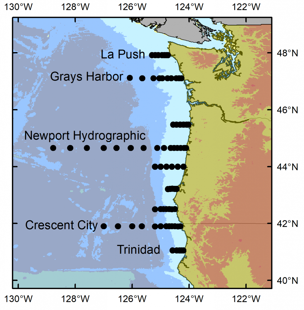
Clara and I have just returned from ten fruitful days at sea aboard NOAA Ship Bell M. Shimada as part of the Northern California Current (NCC) ecosystem survey. We surveyed between Crescent City, California and La Push, Washington, collecting data on oceanography, phytoplankton, zooplankton, and marine mammals (Fig. 1). This year represents the third year I have participated in these NCC cruises, which I have come to cherish. I have become increasingly confident in my marine mammal observation and species identification skills, and I have become more accepting of the things out of my control – the weather, the sea state, the many sightings of “unidentified whale species”. Careful planning and preparation are critical, and yet out at sea we are ultimately at the whim of the powerful Pacific Ocean. Another aspect of the NCC cruises that I treasure is the time spent with members of the science team from other disciplines. The chatter about water column features, musings about plankton species composition, and discussions about what drives marine mammal distribution present lively learning opportunities throughout the cruise. Our concurrent data collection efforts and ongoing conversations allow us to piece together a comprehensive picture of this dynamic NCC ecosystem, and foster a collaborative research environment.
Figure 1. Data collection effort for the NCC September 2020 cruise, between Crescent City, CA, and La Push, WA. Red points represent oceanographic sampling stations, and black lines show the track of the research vessel during marine mammal survey effort.
Every time I head to sea, I am reminded of the patchy distribution of resources in the vast and dynamic marine environment. On this recent cruise we documented a stark contrast between expansive stretches of warm, blue, stratified, and seemingly empty ocean and areas that were plankton-rich and supported multi-species feeding frenzies that had marine mammal observers like me scrambling to keep track of everything. This year, we were greeted by dozens of blue and humpback whales in the productive waters off Newport, Oregon. Off Crescent City, California, the water was very warm, the plankton community was dominated by gelatinous species like pyrosomes, salps, and other jellies, and the marine mammals were virtually absent except for a few groups of common dolphins. To the north, the plume of water flowing from the Columbia River created a front between water masses, where we found ourselves in the midst of pacific white-sided dolphins, northern right whale dolphins, and humpback whales. These observations highlight the strength of ecosystem-scale and multi-disciplinary data collection efforts such as the NCC surveys. By drawing together information on physical oceanography, primary productivity, zooplankton community composition and abundance, and marine predator distribution, we can gain a nearly comprehensive picture of the dynamics within the NCC over a broad spatial scale.
Northern fur seal
Humpback whales
Common dolphins
Humpback whale breaching
Blue whale
Risso’s dolphins
Pacific white-sided dolphins
A few images of marine mammals of the NCC. Click a photo to explore gallery. All photos by Dawn Barlow.
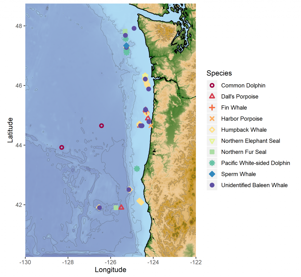
This year, the marine mammals delivered and kept us observers busy. We lucked out with good survey conditions and observed many different species throughout the NCC (Table 1, Fig. 2).
Table 1. Summary of all marine mammal sightings from the NCC September 2020 cruise.
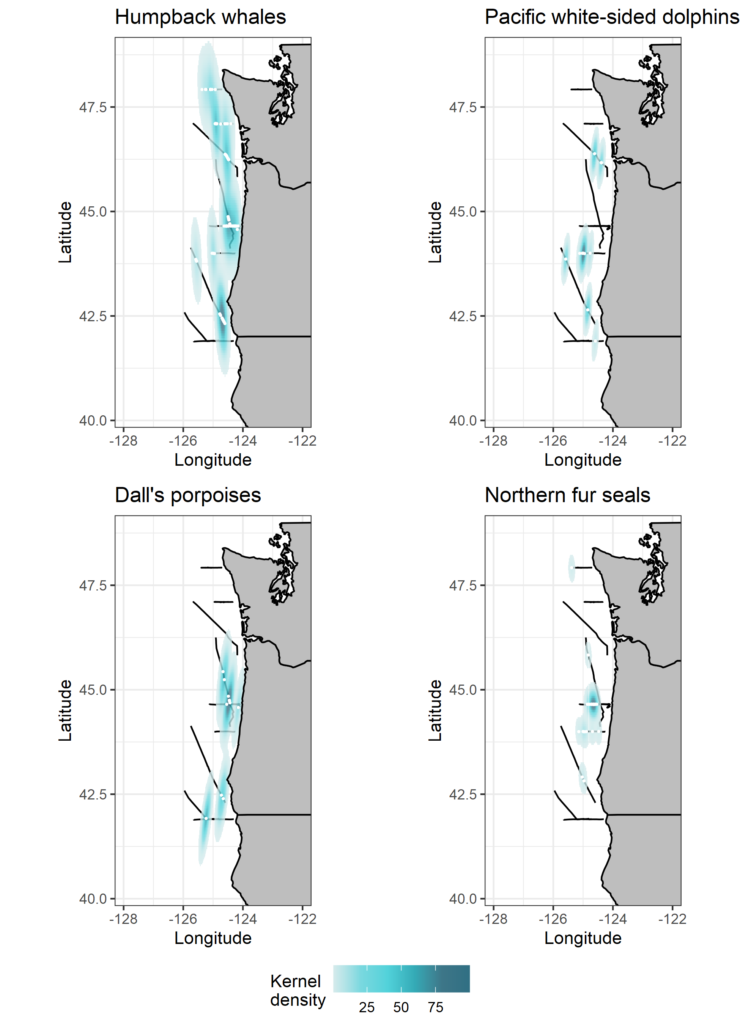
Figure 2. Maps showing kernel densities of four frequently observed and widely distributed species seen during the cruise. Black lines show the track of the research vessel during marine mammal survey effort, white points represent sighting locations, and colors show kernel density estimates weighted by group size at each sighting.
This year’s NCC cruise was unique. We went to sea as a global pandemic, wildfires, and political tensions continue to strain this country and our communities. This cruise was the first NOAA Fisheries cruise to set sail since the start of the pandemic. Our team of scientists and the ship’s crew went to great lengths to make it possible, including a seven-day shelter-in-place period and COVID-19 tests prior to cruise departure. As a result of these extra challenges and preparations, I think we were all especially grateful to be on the water, collecting data. At-sea fieldwork is always challenging, but morale was up, spirits were high, and laughs were frequent despite smiles being concealed by our masks. I am grateful for the opportunity to participate in this ongoing valuable data collection effort, and to be part of this team. Thanks to all who made it such a memorable cruise.
Figure 3. The NCC September 2020 science team at the end of a successful research cruise! Fieldwork in the time of COVID-19 presents many logistical challenges, but this team rose to the occasion and completed a safe and fruitful survey despite the circumstances.
Clara Bird, Masters Student, OSU Department of Fisheries and Wildlife, Geospatial Ecology of Marine Megafauna Lab
The GEMM Lab gray whale team is in the midst of preparing for our fifth field season studying the Pacific Coast Foraging Group (PCFG): whales that forage off the coast of Newport, OR, USA each summer. On any given good weather day from June to October, our team is out on the water in a small zodiac looking for gray whales (Figure 1). When we find a gray whale, we try to collect photo ID data, fecal samples, drone data, and behavioral data. We use the drone data to study both the whale’s body condition and their behavior. In a previous blog, I described ethograms and how I would like to use the behavior data from drone videos to classify behaviors, with the ultimate goal of understanding how gray whale behavior varies across space, time, and by individual. However, this explanation of studying whale behavior is actually a bit incomplete. Before we start fieldwork, we first need to decide how to collect that data.
Figure 1. Image of GEMM lab team collecting gray whale UAS data. Image taken under NOAA/NMFS permit #16111
As observers, we are far from omnipresent and there is no way to know what the animals are doing all of the time. In any environment, scientists have to decide when and where to observe their animals and what behaviors they are interested in recording. In many studies, behavior is recorded live by an observer. In those studies, other limitations need to be taken into account, such as human error and observer fatigue. Collecting behavioral data is particularly challenging in the marine environment. Cetaceans spend most of their lives out of sight from humans, their time at the surface is brief, and when they appear together in large groups it can be very difficult to keep track of who is doing what when. Imagine being in a boat trying to keep track of what three different whales are doing without a pre-determined method – the task could quickly become overwhelming and biased. This is why we need a methodology for collecting and classifying behavior. We cannot study behavior without acknowledging these limitations and the potential biases that come with the methods we choose. Different data collection methods are better suited to address different questions.
The use of drones gives us the ability to record cetacean behavior non-invasively, from a perspective that allows greater observation (Figure 2, Torres et al. 2018), and for later review, which is a significant improvement. However, as we prepare to collect more behavior data, we need to study the methods and understand the benefits and disadvantages of each approach so that we capture the information we need without bias. Altmann (1974) provides a thorough overview of behavioral sampling methods.
Figure 2. Diagram illustrating “whale surface time” relative to “whale visible time” data as collected from an unmanned aerial systems (UAS) aircraft flying over a gray whale as it moves sequentially (from right to left) from “headstand” foraging to surfacing. Figure from Torres et al. (2018).
Ad libitum behavioral sampling has no structure and occurs when we find a group of whales and just write down everything they are doing. This method is a good first step, however it comes with bias. Without structure, we cannot be sure that there was an equal probability of detecting each kind of behavior; this problem is called detectability bias. This type of bias is an issue if we are trying to answer questions about how often a behavior occurs, or what percent of time is spent in each behavior state. This is a bias to be especially concerned about when it comes to cetaceans because there are many examples of behaviors with different levels of detectability. An extreme example would be the detectability of breaching versus a behavior that takes place under the surface. A breaching whale is easier to spot and more exciting, which could lead to results suggesting that whales breach more often than they do relative to underwater behaviors. While it’s impossible to eliminate detectability bias, other sampling methods employ decision rules to try and reduce its effect. Many decision rules revolve around time, such as setting a minimum or maximum observation time interval. Other time rules involve recording the behavior state at set intervals of time (e.g., every 5 minutes). Setting observation boundaries helps standardize the methods and the data being collected.
In a structured sampling plan, the first big decision that needs to be addressed is the need to know the duration of behaviors. Point events do not include duration data but can be used to study the frequencies of behaviors. For example, if my research question was “Do whales perform “headstands” in a specific habitat type?”, then I would need point events of headstanding behavior. But, if I wanted to ask, “Do whales spend more time spent headstanding in a specific habitat type than in other habitat types?”, I would need headstanding to be a state event. State events are events with associated duration information and can be used for activity budgets. Activity budgets show how much time an animal spends in each behavior state. Some sampling methods focus on collecting only point events. However, to get the most complete understanding of behavior I think it’s important to collect both. Focal animal follows are another method of collecting more detailed data and is commonly used in cetacean studies.
The explanation of a focal follow method is in the name. We focus on one individual, follow it, and record all of its behaviors. When employing this method, decisions are made about how an individual is chosen and how long it is followed. In some cases, the behavior of this animal is used as a proxy for the behavior of an entire group. I essentially use the focal follow method in my research. While I review drone footage to record behavioral data instead of recording behaviors live in the field, I focus on one individual a time as I go through the videos. To do this I use a software called BORIS (Friard and Gamba 2016) to mark the time of each behavior per individual (Figure 3). If there are three individuals in a video, I’ll review the footage three times to record behaviors once per individual, focusing on each in turn.
Figure 3. Screenshot of BORIS layout.
While the drone footage brings the advantages of time to review and a better view of the whale, we are constrained by the duration of a flight. Focal follows would ideally last longer than the ~15 minutes of battery life per drone flight. Our previously collected footage gives us snapshots of behavior, and this makes it challenging to compare and analyze durations of behaviors. Therefore, I am excited that we are going to try conducting drone focal follows this summer by swapping out drones when power runs low to achieve longer periods of video coverage of whale behavior. I’ll be able to use these data to move from snapshots to analyzing longer clips and better understanding the behavioral ecology of gray whales. As exciting as this opportunity is, it also presents the challenge of method development. So, I now need to develop decision rules and data collection methods to answer the questions that I have been eagerly asking.
Friard, Olivier, and Marco Gamba. 2016. “BORIS: A Free, Versatile Open-Source Event-Logging Software for Video/Audio Coding and Live Observations.” Methods in Ecology and Evolution 7 (11): 1325–30. https://doi.org/10.1111/2041-210X.12584.
Torres, Leigh G., Sharon L. Nieukirk, Leila Lemos, and Todd E. Chandler. 2018. “Drone up! Quantifying Whale Behavior from a New Perspective Improves Observational Capacity.” Frontiers in Marine Science 5 (SEP). https://doi.org/10.3389/fmars.2018.00319.
There is something wonderful about time at sea, where your primary obligation is to observe the ocean from sunrise to sunset, day after day, scanning for signs of life. After hours of seemingly empty blue with only an occasional albatross gliding over the swells on broad wings, it is easy to question whether there is life in the expansive, blue, offshore desert. Splashes on the horizon catch your eye, and a group of dolphins rapidly approaches the ship in a flurry of activity. They play in the ship’s bow and wake, leaping out of the swells. Then, just as quickly as they came, they move on. Back to blue, for hours on end… until the next stirring on the horizon. A puff of exhaled air from a whale that first might seem like a whitecap or a smudge of sunscreen or salt spray on your sunglasses. It catches your eye again, and this time you see the dark body and distinctive dorsal fin of a humpback whale.
Figure 1. Pacific white-sided dolphins (Lagenorhynchus obliquidens) play in the big swell and surf the wake of the NOAA ship Bell M. Shimada off Coos Bay, Oregon. Photos: Dawn Barlow.
I have just returned from 10 days aboard the NOAA ship Bell M. Shimada, where I was the marine mammal observer on the Northern California Current (NCC) Cruise. These research cruises have sampled the NCC in the winter, spring, and fall for decades. As a result, a wealth of knowledge on the oceanography and plankton community in this dynamic ocean ecosystem has been assimilated by a dedicated team of scientists (find out more via the Newportal Blog). Members of the GEMM Lab have joined this research effort in the past two years, conducting marine mammal surveys during the transits between sampling stations (Fig. 2).
Figure 2. Northern California Current cruise sampling locations, where oceanography and plankton data are collected. Marine mammal surveys were conducted on the transits between stations.
The fall 2019 NCC cruise was a resounding success. We were able to survey a large swath of the ecosystem between Crescent City, CA and La Push, WA, from inshore to 200 miles offshore. During that time, I observed nine different species of marine mammals (Table 1). As often as I use some version of the phrase “the marine environment is patchy and dynamic”, it never fails to sink in a little bit more every time I go to sea. On the map in Fig. 3, note how clustered the marine mammal sightings are. After nearly a full day of observing nothing but blue water, I would find myself scrambling to keep up with recording all the whales and dolphins we were suddenly in the midst of. What drives these clusters of sightings? What is it about the oceanography and prey community that makes any particular area a hotspot for marine mammals? We hope to get at these questions by utilizing the oceanographic data collected throughout the surveys to better understand environmental drivers of these distribution patterns.
Table 1. Summary of marine mammal
sightings from the September 2019 NCC Cruise.
Species
# sightings
Total # individuals
Northern Elephant Seal
1
1
Northern Fur Seal
2
2
Common Dolphin
2
8
Pacific White-sided Dolphin
8
143
Dall’s Porpoise
4
19
Harbor Porpoise
1
3
Sperm Whale
1
1
Fin Whale
1
1
Humpback Whale
22
36
Unidentified Baleen Whale
14
16
Figure 3. Map of marine mammal sighting locations from the September NCC cruise.
It was an auspicious time to survey the Northern California Current. Perhaps you have read recent news reports warning about the formation of another impending marine heatwave, much like the “warm blob” that plagued the North Pacific in 2015. We experienced it first-hand during the NCC cruise, with very warm surface waters off Newport extending out to 200 miles offshore (Fig. 4). A lot of energy input from strong winds would be required to mix that thick, warm layer and allow cool, nutrient-rich water to upwell along the coast. But it is already late September, and as the season shifts from summer to fall we are at the end of our typical upwelling season, and the north winds that would typically drive that mixing are less likely. Time will tell what is in store for the NCC ecosystem as we face the onset of another marine heatwave.
Figure 4. Temperature contours over the upper 150 m from 1-200 miles off Newport, Oregon from Fall 2014-2019. During Fall 2014, the Warm Blob inundated the Oregon shelf. Surface temperatures during that survey were 17°- 18°C along the entire transect. During 2015 and 2016 the warm water (16°C) layer had deepened and occupied the upper 50 m. During 2018, the temperature was 16°C in the upper 20 m and cooler on the shelf, indicative of residual upwelling. During this survey in 2019, we again saw very warm (18°C) temperatures in the upper water column over the entire transect. Image and caption credit: Jennifer Fisher.
It was a joy to spend 10 days at sea with this team of scientists. Insight, collaboration, and innovation are born from interdisciplinary efforts like the NCC cruises. Beyond science, what a privilege it is to be on the ocean with a group of people you can work with and laugh with, from the dock to 200 miles offshore, south to north and back again.
Dawn Barlow on the flying bridge of NOAA Ship Bell M. Shimada, heading out to sea with the Newport bridge in the background. Photo: Anna Bolm.
By Leila Lemos, PhD Candidate, Fisheries and Wildlife Department, Oregon State University
After three years of fieldwork and analyzing a large dataset, it is time to finally start compiling the results, create plots and see what the trends are. The first dataset I am analyzing is the photogrammetry data (more on our photogrammetry method here), which so far has been full of unexpected results.
Our first big expectation was to find a noticeable intra-year variation. Gray whales spend their winter in the warm waters of Baja California, Mexico, period while they are fasting. In the spring, they perform a big migration to higher latitudes. Only when they reach their summer feeding grounds, that extends from Northern California to the Bering and Chukchi seas, Alaska, do they start feeding and gaining enough calories to support their migration back to Mexico and subsequent fasting period.
Northeastern gray whale migration route along the NE Pacific Ocean. Source: https://journeynorth.org/tm/gwhale/annual/map.html
Thus, we expected to see whales arriving along the Oregon coast with a skinny body condition that would gradually improve over the months, during the feeding season. Some exceptions are reasonable, such as a lactating mother or a debilitated individual. However, datasets can be more complex than we expect most of the times, and many variables can influence the results. Our photogrammetry dataset is no different!
In addition, I need to decide what are the best plots to display the results and how to make them. For years now I’ve been hearing about the wonders of R, but I’ve been skeptical about learning a whole new programming/coding language “just to make plots”, as I first thought. I have always used statistical programs such as SPSS or Prism to do my plots and they were so easy to work with. However, there is a lot more we can do in R than “just plots”. Also, it is not just because something seems hard that you won’t even try. We need to expose ourselves sometimes. So, I decided to give it a try (and I am proud of myself I did), and here are some of the results:
Plot 1: Body Area Index (BAI) vs Day of the Year (DOY)
In this plot, we wanted to assess the annual Body Area Index (BAI) trends that describe how skinny (low number) or fat (higher number) a whale is. BAI is a simplified version of the BMI (Body Mass Index) used for humans. If you are interested about this method we have developed at our lab in collaboration with the Aerial Information Systems Laboratory/OSU, you can read more about it in our publication.
The plots above are three versions of the same data displayed in different ways. The first plot on the left shows all the data points by year, with polynomial best fit lines, and the confidence intervals (in gray). There are many overlapping observation points, so for the middle plot I tried to “clean up the plot” by reducing the size of the points and taking out the gray confidence interval range around the lines. In the last plot on the right, I used a linear regression best fit line, instead of polynomial.
We can see a general trend that the BAI was considerably higher in 2016 (red line), when compared to the following years, which makes us question the accuracy of the dataset for that year. In 2016, we also didn’t sample in the month of July, which is causing the 2016 polynomial line to show a sharp decrease in this month (DOY: ~200-230). But it is also interesting to note that the increasing slope of the linear regression line in all three years is very similar, indicating that the whales gained weight at about the same rate in all years.
Plot 2: Body Area Index (BAI) vs Body Condition Score (BCS)
In addition to the photogrammetry method of assessing whale body condition, we have also performed a body condition scoring method for all the photos we have taken in the field (based on the method described by Bradford et al. 2012). Thus, with this second set of plots, we wanted to compare both methods of assessing whale body condition in order to evaluate when the methods agree or not, and which method would be best and in which situation. Our hypothesis was that whales with a ‘fair’ body condition would have a lower BAI than whales with a ‘good’ body condition.
The plots above illustrate two versions of the same data, with data in the left plot grouped by year, and the data in the right plot grouped by month. In general, we see that no whales were observed with a poor body condition in the last analysis months (August to October), with both methods agreeing to this fact. Additionally, there were many whales that still had a fair body condition in August and September, but less whales in the month of October, indicating that most whales gained weight over the foraging seasons and were ready to start their Southbound migration and another fasting period. This result is important information regarding monitoring and conservation issues.
However, the 2016 dataset is still a concern, since the whales appear to have considerable higher body condition (BAI) when compared to other years.
Plot 3:Temporal Body Area Index (BAI) for individual whales
In this last group of plots, we wanted to visualize BAI trends over the season (using day of year – DOY) on the x-axis) for individuals we measured more than once. Here we can see the temporal patterns for the whales “Bit”, “Clouds”, “Pearl”, “Scarback, “Pointy”, and “White Hole”.
We expected to see an overall gradual increase in body condition (BAI) over the seasons, such as what we can observe for Pointy in 2018. However, some whales decreased their condition, such as Bit in 2018. Could this trend be accurate? Furthermore, what about BAI measurements that are different from the trend, such as Scarback in 2017, where the last observation point shows a lower BAI than past observation points? In addition, we still observe a high BAI in 2016 at this individual level, when compared to the other years.
My next step will be to check the whole dataset again and search for inconsistencies. There is something causing these 2016 values to possibly be wrong and I need to find out what it is. The overall quality of the measured photogrammetry images was good and in focus, but other variables could be influencing the quality and accuracy of the measurements.
For instance, when measuring images, I often struggled with glare, water splash, water turbidity, ocean swell, and shadows, as you can see in the photos below. All of these variables caused the borders of the whale body to not be clearly visible/identifiable, which may have caused measurements to be wrong.
Examples of bad conditions for performing photogrammetry: (1) glare and water splash, (2) water turbidity, (3) ocean swell, and (4) a shadow created in one of the sides of the whale body. Source: GEMM Lab. Taken under NMFS permit 16111 issued to John Calambokidis.
Thus, I will need to check all of these variables to identify the causes for bad measurements and “clean the dataset”. Only after this process will I be able to make these plots again to look at the trends (which will be easy since I already have my R code written!). Then I’ll move on to my next hypothesis that the BAI of individual whales varied by demographics including sex, age and reproductive state.
To carry out robust science that produces results we can trust, we can’t simply collect data, perform a basic analysis, create plots and believe everything we see. Data is often messy, especially when developing new methods like we have done here with drone based photogrammetry and the BAI. So, I need to spend some important time checking my data for accuracy and examining confounding variables that might affect the dataset. Science can be challenging, both when interpreting data or learning a new command language, but it is all worth it in the end when we produce results we know we can trust.
By Alexa Kownacki, Ph.D. Student, OSU Department of Fisheries and Wildlife, Geospatial Ecology of Marine Megafauna Lab
From September 22nd through 30th, the GEMM Lab participated in a STEM research cruise aboard the R/V Oceanus, Oregon State University’s (OSU) largest research vessel, which served as a fully-functioning, floating, research laboratory and field station. The STEM cruise focused on integrating science, technology, engineering and mathematics (STEM) into hands-on teaching experiences alongside professionals in the marine sciences. The official science crew consisted of high school teachers and students, community college students, and Oregon State University graduate students and professors. As with a usual research cruise, there was ample set-up, data collection, data entry, experimentation, successes, and failures. And because everyone in the science party actively participated in the research process, everyone also experienced these successes, failures, and moments of inspiration.
The science party enjoying the sunset from the aft deck with the Astoria-Megler bridge in the background. (Image source: Alexa Kownacki)
Dr. Leigh Torres, Dr. Rachael Orben, and I were all primarily stationed on flybridge—one deck above the bridge—fully exposed to the elements, at the highest possible location on the ship for best viewing. We scanned the seas in hopes of spotting a blow, a splash, or any sign of a marine mammal or seabird. Beside us, students and teachers donned binoculars and positioned themselves around the mast, with Leigh and I taking a 90-degree swath from the mast—either to starboard or to port. For those who had not been part of marine mammal observations previously, it was a crash course into the peaks and troughs—of both the waves and of the sightings. We emphasized the importance of absence data: knowledge of what is not “there” is equally as important as what is. Fortunately, Leigh chose a course that proved to have surprisingly excellent environmental conditions and amazing sightings. Therefore, we collected a large amount of presence data: data collected when marine mammals or seabirds are present.
High school student, Chris Quashnick Holloway, records a seabird sighting for observer, Dr. Rachael Orben. (Image source: Alexa Kownacki).
When someone sighted a whale that surfaced regularly, we assessed the conditions: the sea state, the animal’s behavior, the wind conditions, etc. If we deemed them as “good to fly”, our licensed drone pilot and Orange Coast Community College student, Jason, prepared his Phantom 4 drone. While he and Leigh set up drone operations, I and the other science team members maintained a visual on the whale and stayed in constant communication with the bridge via radio. When the drone was ready, and the bridge gave the “all clear”, Jason launched his drone from the aft deck. Then, someone tossed an unassuming, meter-long, wood plank overboard—keeping it attached to the ship with a line. This wood board serves as a calibration tool; the drone flies over it at varying heights as determined by its built-in altimeter. Later, we analyze how many pixels one meter occupied at different heights and can thereby determine the body length of the whale from still images by converting pixel length to a metric unit.
High school student, Alishia Keller, uses binoculars to observe a whale, while PhD student, Alexa Kownacki, radios updates on the whale’s location to the bridge and the aft deck. (Image source: Tracy Crews)
Finally, when the drone is calibrated, I radio the most recent location of our animal. For example, “Blow at 9 o’clock, 250 meters away”. Then, the bridge and I constantly adjust the ship’s speed and location. If the whale “flukes” (dives and exposes the ventral side of its tail), and later resurfaced 500 meters away at our 10 o’clock, I might radio to the bridge to, “turn 60 degrees to port and increase speed to 5 knots”. (See the Hidden Math Lesson below). Jason then positions the drone over the whale, adjusting the camera angle as necessary, and recording high-quality video footage for later analysis. The aerial viewpoint provides major advantages. Whales usually expose about 10 percent of their body above the water’s surface. However, with an aerial vantage point, we can see more of the whale and its surroundings. From here, we can observe behaviors that are otherwise obscured (Torres et al. 2018), and record footage that to help quantify body condition (i.e. lengths and girths). Prior to the batteries running low, Jason returns the drone back to the aft deck, the vessel comes to an idle, and Leigh catches the drone. Throughout these operations, those of us on the flybridge photograph flukes for identification and document any behaviors we observe. Later, we match the whale we sighted to the whale that the drone flew over, and then to prior sightings of this same individual—adding information like body condition or the presence of a calf. I like to think of it as whale detective work. Moreover, it is a team effort; everyone has a critical role in the mission. When it’s all said and done, this noninvasive approach provides life history context to the health and behaviors of the animal.
Drone pilot, Jason Miranda, flying his drone using his handheld ground station on the aft deck. (Photo source: Tracy Crews)
Hidden Math Lesson: The location of 10 o’clock and 60 degrees to port refer to the exact same direction. The bow of the ship is our 12 o’clock with the stern at our 6 o’clock; you always orient yourself in this manner when giving directions. The same goes for a compass measurement in degrees when relating the direction to the boat: the bow is 360/0. An angle measure between two consecutive numbers on a clock is: 360 degrees divided by 12-“hour” markers = 30 degrees. Therefore, 10 o’clock was 0 degrees – (2 “hours”)= 0 degrees- (2*30 degrees)= -60 degrees. A negative degree less than 180 refers to the port side (left).
Killer whale traveling northbound.
Our trip was chalked full of science and graced with cooperative weather conditions. There were more highlights than I could list in a single sitting. We towed zooplankton nets under the night sky while eating ice cream bars; we sang together at sunset and watched the atmospheric phenomena: the green flash; we witnessed a humpback lunge-feeding beside the ship’s bow; and we saw a sperm whale traveling across calm seas.
Sperm whale surfacing before a long dive.
On this cruise, our lab focused on the marine mammal observations—which proved excellent during the cruise. In only four days of surveying, we had 43 marine mammal sightings containing 362 individuals representing 9 species (See figure 1). As you can see from figure 2, we traveled over shallow, coastal and deep waters, in both Washington and Oregon before inland to Portland, OR. Because we ventured to areas with different bathymetric and oceanographic conditions, we increased our likelihood of seeing a higher diversity of species than we would if we stayed in a single depth or area.
Humpback whale lunge feeding off the bow.
Number of sightings
Total number of individuals
Humpback whale
22
40
Pacific white-sided dolphin
3
249
Northern right whale dolphin
1
9
Killer whale
1
3
Dall’s porpoise
5
49
Sperm whale
1
1
Gray whale
1
1
Harbor seal
1
1
California sea lion
8
9
Total
43
362
Figure 1. Summary table of all species sightings during cruise while the science team observed from the flybridge.
Pacific white-sided dolphins swimming towards the vessel.
Figure 2. Map with inset displaying study area and sightings observed by species during the cruise, made in ArcMap. (Image source: Alexa Kownacki).
Even after two days of STEM outreach events in Portland, we were excited to incorporate more science. For the transit from Portland, OR to Newport, OR, the entire science team consisted two people: me and Jason. But even with poor weather conditions, we still used science to answer questions and help us along our journey—only with different goals than on our main leg. With the help of the marine technician, we set up a camera on the bow of the ship, facing aft to watch the vessel maneuver through the famous Portland bridges.
Video 1. Time-lapse footage of the R/V Oceanus maneuvering the Portland Bridges from a GoPro. Compiled by Alexa Kownacki, assisted by Jason Miranda and Kristin Beem.
Prior to the crossing the Columbia River bar and re-entering the Pacific Ocean, the R/V Oceanus maneuvered up the picturesque Columbia River. We used our geospatial skills to locate our fellow science team member and high school student, Chris, who was located on land. We tracked each other using GPS technology in our cell phones, until the ship got close enough to use natural landmarks as reference points, and finally we could use our binoculars to see Chris shining a light from shore. As the ship powered forward and passed under the famous Astoria-Megler bridge that connects Oregon to Washington, Chris drove over it; he directed us “100 degrees to port”. And, thanks to clear directions, bright visual aids, and spatiotemporal analysis, we managed to find our team member waving from shore. This is only one of many examples that show how in a few days at sea, students utilized new skills, such as marine mammal observational techniques, and honed them for additional applications.
On the bow, Alexa and Jason use binoculars to find Chris–over 4 miles–on the Washington side of the Columbia River. (Image source: Kristin Beem)
Great science is the result of teamwork, passion, and ingenuity. Working alongside students, teachers, and other, more-experienced scientists, provided everyone with opportunities to learn from each other. We created great science because we asked questions, we passed on our knowledge to the next person, and we did so with enthusiasm.
High school students, Jason and Chris, alongside Dr. Leigh Torres, all try to get a glimpse at the zooplankton under Dr. Kim Bernard’s microscope. (Image source: Tracy Crews).
Check out other blog posts written by the science team about the trip here.