New publication reveals gray whale habitat use patterns over three decades in the Northern California Current

By Dr. Dawn Barlow, Postdoctoral Scholar, OSU Department of Fisheries, Wildlife, and Conservation Sciences, Geospatial Ecology of Marine Megafauna Lab

The EMERALD project (Examining Marine mammal Ecology through Regional Assessment of Long-term Data) has reached a milestone with a recent publication detailing our findings on long-term gray whale distribution, abundance, and habitat use patterns (Barlow et al. 2024). The study is made possible by an incredible dataset. Every May-July since 1992, a team of observers surveyed the coastline between the Columbia River at the border between Oregon and Washington and San Francisco Bay, California for marbled murrelets, a seabird species of conservation concern. They drive a small vessel along pre-determined tracklines, and record observations of seabirds and marine mammals—not just marbled murrelets—and fortunately for us, that means there is a record of annual gray whale distribution and abundance patterns that spans over three decades.

The Crescent Coastal Research team collecting survey data. We are incredibly grateful to Craig Strong and the many folks who collected these valuable observations over the years!

We analyzed these valuable data using density surface modeling to better understand what drives gray whale distribution and abundance, what their habitat preferences are, and whether and how these occurrence patterns have changed over time. I am excited to share a few of our findings here!

Long-term, stable hotspots

The survey data revealed three main areas with consistently high gray whale density: the central Oregon Coast off Newport, Cape Blanco off Oregon’s south coast, and the mouth of the Klamath River in northern California. Despite fluctuations in how many whales were observed over the years, these areas have remained predicable hotspots for gray whales during their summer feeding season.

(A) Mean gray whale encounter rate (whales/kilometers surveyed) summarized by year, across all latitudes. (B) Mean gray whale encounter rate summarized by 1° latitude bin, across all years. White indicates times and locations with no survey effort. (C) Mean gray whale encounter rate summarized by year and 1° latitude bin. (D) Map of the study area, with region boundaries shown by the dashed lines, and major placenames denoted. Figure and caption reproduced from Barlow et al. 2024.

Key regional differences

Major features like prominent capes divide the California Current into different regions with distinct oceanographic characteristics. We found that gray whales showed different habitat preferences in the different regions. In the northern part of our study area between the Columbia River and Cape Blanco, we found that rocky bottom substrate was strongly related to areas of higher gray whale abundance, despite being far less available than soft, sandy bottom habitat. In the region between Cape Blanco and Cape Mendocino, gray whales were more abundant in areas south of prominent capes and in closer proximity to river estuaries.

Coastal upwelling and relaxation are key

Coastal upwelling—the process by which winds in the spring and summer push surface water offshore that is then replaced by cold, nutrient-rich water that is brought into the sunlight and drives an abundance of marine life—is a critically important influence in the oceanography, ecology, and biodiversity of our study region. But relaxation of those upwelling winds is also important for coastal species, as relaxation events allow the upwelled nutrients to be retained in the nearshore waters and enhance and aggregate local productivity and prey. We found that gray whale abundance was highest when there was a combination of both upwelling and relaxation events—a critical balance of “enough but not too much”—that seems to be optimal for gray whale feeding opportunities in nearshore waters.

You are what, where, and how you eat

Gray whales are incredibly flexible predators and have a wide range of prey items they are known to feed on. We found that throughout our study range, gray whales have different habitat preferences. As they spend their summers here to feed, these habitat preferences are linked to their foraging preferences. Off the central Oregon Coast, gray whales are known to feed on zooplankton that aggregate around rocky reefs and kelp forests (Hildebrand et al. 2022, 2024).

A gray whale surfaces in a patch of kelp, foraging around a rocky reef. UAS image credit: GEMM Lab.

Further south, in the region between Cape Blanco and Cape Mendocino that encompassed the long-term hotspot of gray whale sightings off the Klamath River, our models revealed different habitat preferences. In the soft-bottom habitat off the Klamath River, gray whales are known to do more benthic feeding, whereby they scoop up the seafloor and filter out the invertebrates in the sediment such as amphipods and cumaceans (Mallonée 1991, Jenkinson 2001).

A gray whale surfaces with a mouth full of muddy sediment, filtering out the invertebrate prey. UAS image credit: GEMM Lab.

These differences in regional habitat preferences and preferred prey likely relate to larger-scale phenomena as well. Indeed, when we looked at how gray whale abundance in different regions related to widespread warm or cool phases in the North Pacific Ocean, the responses differed by region. This aspect of the study indicates that what gray whales eat and where they forage influences how they respond to shifting environmental conditions and prey availability.

Conservation of an iconic nearshore predator

The unique mosaic of habitat characteristics throughout the Northern California Current summer feeding range of gray whales provides them the opportunity to gain the energetic stores they need to survive, reproduce, and migrate. Thus, the reliability of these resources has led them to return to these stable foraging hotspots year after year. Under climate change, one potential impact on upwelling systems is shifts in the intensity and location of upwelling (Bograd et al. 2023); in the Northern California Current, this could mean reduced relaxation events that we found are crucial for gray whales feeding in this habitat. Furthermore, these whales overlap with human activities such as vessel disturbance, entanglement and vessel strike risk, and ocean noise throughout the foraging season, and have to bear the consequences of these anthropogenic stressors (Sullivan & Torres 2018, Lemos et al. 2022, Pirotta et al. 2023) as they also navigate changing environmental conditions. Our study highlights the value of long-term monitoring to better understand present ecological patterns in the context of the past, which can be used to inform conservation management decisions for the future.

For more details, we invite you to read the full, open access publication here: https://www.nature.com/articles/s41598-024-59552-z

Did you enjoy this blog? Want to learn more about marine life, research, and conservation? Subscribe to our blog and get a weekly alert when we make a new post! Just add your name into the subscribe box below!

Loading

References

Barlow DR, Strong CS, Torres LG (2024) Three decades of nearshore surveys reveal long-term patterns in gray whale habitat use, distribution, and abundance in the Northern California Current. Sci Rep 14:9352.

Bograd SJ, Jacox MG, Hazen EL, Lovecchio E, Montes I, Pozo Buil M, Shannon LJ, Sydeman WJ, Rykaczewski RR (2023) Climate Change Impacts on Eastern Boundary Upwelling Systems. Ann Rev Mar Sci 15:1–26.

Hildebrand L, Derville S, Hildebrand I, Torres LG (2024) Exploring indirect effects of a classic trophic cascade between urchins and kelp on zooplankton and whales. Sci Rep 14.

Hildebrand L, Sullivan FA, Orben RA, Derville S, Torres LG (2022) Trade-offs in prey quantity and quality in gray whale foraging. Mar Ecol Prog Ser 695:189–201.

Jenkinson RS (2001) Gray whale (Eschrichtius robustus) prey availability and feeding ecology in Northern California, 1999-2000. Humboldt State University

Lemos L, Haxel J, Olsen A, Burnett JD, Smith A, Chandler TE, Nieukirk SL, Larson SE, Hunt KE, Torres LG (2022) Effects of vessel traffic and ocean noise on gray whale stress hormones. Sci Rep 12:1–13.

Mallonée JS (1991) Behaviour of gray whales (Eschrichtius robustus) summering off the northern California coast, from Patrick’s Point to Crescent City. Can J Zool 69:681–690.

Pirotta E, Fernandez Ajó A, Bierlich KC, Bird CN, Buck CL, Haver SM, Haxel JH, Hildebrand L, Hunt KE, Lemos LS, New L, Torres LG (2023) Assessing variation in faecal glucocorticoid concentrations in gray whales exposed to anthropogenic stressors. Conserv Physiol 11:coad082.

Sullivan FA, Torres LG (2018) Assessment of vessel disturbance to gray whales to inform sustainable ecotourism. J Wildl Manage 82:896–905.

Rorquals of the California Current

By Solène Derville, Postdoc, OSU Department of Fisheries, Wildlife, and Conservation Science, Geospatial Ecology of Marine Megafauna Lab

About 10 months have passed since I started working on OPAL, a project that aims to identify the co-occurrence between whales and fishing effort in Oregon to reduce entanglement risk. During this period, you would be surprised to know how little ecology I have actually done and how much time has been devoted to data processing! I compiled several million GPS trackline positions, processed hundreds of marine mammal observations, wrote several thousand lines of R code, downloaded and extracted a couple Gb of environmental data… before finally reaching the modeling phase of the OPAL project. And with it, finally comes the time to look more closely at the ecology and behavior of my species of interest. While the previous steps of the project were pretty much devoid of ecological reasoning, the literature homework now comes in handy to guide my choices regarding habitat use models, such as  selecting environmental predictors of whale occurrence, deciding on what seasons should be modeled, and choosing the spatio-temporal scale at which the data should be aggregated.

Whale diversity on the US west coast

The productive waters off the US west coast host a great diversity of cetaceans. Eight species of baleen whales are reported to occur there by NOAA fisheries: blue whales, Bryde’s whales, fin whales, gray whales, humpback whales, minke whales, North Pacific right whales and sei whales. Among them, no less than five are listed as Endangered under the Endangered Species Act. Whether they are only passing by or spending months feeding in the region, the timing and location where these animals are observed varies greatly by species and by population.

During the 113 hours of aerial survey effort and 264 hours of boat-based search conducted for the OPAL project, 563 groups of baleen whales have been observed to-date (up to mid-May 2021 to be exact… more data coming soon!). Among the observations where animals could be identified to the species level, humpback whales are preponderant, as they represent about half of the whale groups observed (n = 293). Blue (n = 41) and gray whales (n = 46) come next, the latter being observed in more nearshore waters. Finally, a few fin whale groups were observed (n = 28). The other baleen whale species reported by NOAA in the US west coast species list were very rarely or not observed at all during OPAL surveys.

The OPAL aerial surveys conducted in partnership with the United States Coast Guard (USCG) were specifically designed to study whales occurring on the continental shelf along the coast of Oregon. Hence, most of this survey effort is located in waters from 800 m to 30 m deep, which may explain the relatively low number of gray whales detected. Indeed, gray whales observed in Oregon may either be migrating along the coast to and from their breeding grounds in Baja California, or be part of the small Pacific Coast Feeding Group that forage in Oregon nearshore and shallow waters during the summer. This group of whales is one the main GEMM lab’s research focus, being at the core of no less than three ongoing research projects: AMBER, GRANITE, and TOPAZ.

So today, let’s turn our eyes to the sea horizon and talk about some other members of the baleen whale community: rorquals. Conveniently, the three species of baleen whales (gray whales aside) most commonly observed during OPAL surveys are all part of the rorqual family, a.k.a Balaenopteridae: humpback whales, blue whales and fin whales (Figure 1). They are morphologically characterized by the pleated throat grooves that allow them to engulf large quantities of food and water, for instance when lunge-feeding. Known cases of hybridization between these three species demonstrate their close relatedness (Jefferson et al., 2021)⁠. They all have worldwide distributions and display unequally understood migratory behaviors, seasonally traveling between warm tropical breeding grounds and temperate-polar feeding grounds. They occur in great numbers in productive waters such as the upwelling system of the California Current.

The three accomplices

Figure 1: Aerial view of three rorquals species: a humpback whale (left), a fin whale (center), and a blue whale (right). Photo credit: Leigh Torres and Craig Hayslip. Photos taken off the Oregon coast under NOAA/NMFS permit during USCG helicopter flights conducted as part of the OPAL project

Humpback whales (Megaptera novaeangliae) are easily differentiated from other rorquals because of their long pectoral fins (up to one third of their body length!), which inspired their scientific name, Megaptera, « big-winged » (Figure 1). Individuals observed in Oregon mostly belong to a mix of two Distinct Population Segments (DPS): the threatened Mexico and endangered Central American DPS. Although humpback whales from different DPS do not show any morphological differences, they are genetically distinct because they have been mating separately in distinct breeding grounds for generations and generations. This genetic differentiation has great implications in terms of conservation since the Central American DPS is recovering at a lesser rate than the Mexican and is therefore subject to different management measures (recovery plan, monitoring plan, designated critical habitats). Humpback whales migrate and feed off the US west coast, with a peak in abundance in the mid to late summer. Compared to other rorquals that are found in the open ocean, humpback whales are mostly observed on the continental shelf (Becker et al., 2019)⁠. They are considered to have a relatively generalist diet, as they feed on a mix of krill (Euphausiids) and fishes (e.g. anchovy, sardines) and are capable of switching their feeding behavior depending on relative prey availability (Fleming, Clark, Calambokidis, & Barlow, 2016; Fossette et al., 2017)⁠.

Blue whales (Balaenoptera musculus) are the largest animals ever known (max length 33 m, Jefferson et al., 2008), and sadly the most at risk of global extinction among our three species of interest (listed as « endangered » in the IUCN red list). They have a distinctive mottled blue and light gray skin, a slender body and a broad U-shaped head (or as some say « like a gothic arch », Figure 1). Blue whales tend to be open ocean animals, but they regroup seasonally to feed in highly productive nearshore areas such as the Southern California Bight (Becker et al. 2019, Abrahms et al. 2019). Blue whales migrating or feeding along the US west coast belong to the Eastern North Pacific stock and are subject to great research and conservation efforts. Contrary to their other rorqual counterparts, blue whales are quite picky eaters, as they exclusively feed on krill. This difference in diet leads to resource partitioning facilitating rorqual coexistence in the California Current (Fossette et al., 2017)⁠. These differences in feeding strategies have important implications for designing predictive models of habitat use.

Fin whales (Balaenoptera physalus) are nicknamed « greyhounds of the sea » due to their exceptional swim speed (max 46 km/h). They are a little smaller than blue whales (max length 27 m, Jefferson, Webber, & Pitman, 2008)⁠ but share a similar sleek and streamlined shape. Their coloration is their most distinctive feature: the left lower jaw being mostly dark while the right is white. V-shaped light-gray « chevrons » color their back, behind the head (Figure 1). The California/Oregon/Washington is one of the three stocks recognized in the North Pacific (NOAA Fisheries, 2018)⁠. Within this region, there is genetic evidence for a geographic separation north and south of Point Conception, CA (Archer et al., 2013)⁠. Like other rorquals, they are migratory, but their seasonal distribution is relatively less well understood as they appear to spend a lot of time in open oceans. For instance, a meta-analysis for the North Pacific found little evidence for fin whales using distinct calving areas (Mizroch, Rice, Zwiefelhofer, Waite, & Perryman, 2009)⁠. In the California Current System, satellite tracking has provided great insights into their space-use patterns. In the Southern California Bight, fin whales show year-round residency and seasonal shifts in habitat use as they move further offshore and north during the spring/summer (Scales et al., 2017)⁠. The Northern California Current offshore waters appeared to be used during the summer months by the whales tagged in the Southern California Bight. Yet, fin whales are observed year-round in Oregon (NOAA Fisheries, 2018)⁠.

Towards predictive models of rorqual distribution

Enough observations have now been collected as part of the OPAL project to be able to model the habitat use of some of these rorqual species. Based on 12 topographic (i.e., depth, slope, distance to canyons) and physical variables (temperature, chlorophyll-a, water column stratification, etc.), I have made my first attempt at predicting seasonal distribution patterns of humpback whales and blue whales in Oregon. These models will be improved in the coming months, with more data pouring in and refined parametrizations, but they already bring insights into the shared habitat use patterns of these species, as well as their specificities.

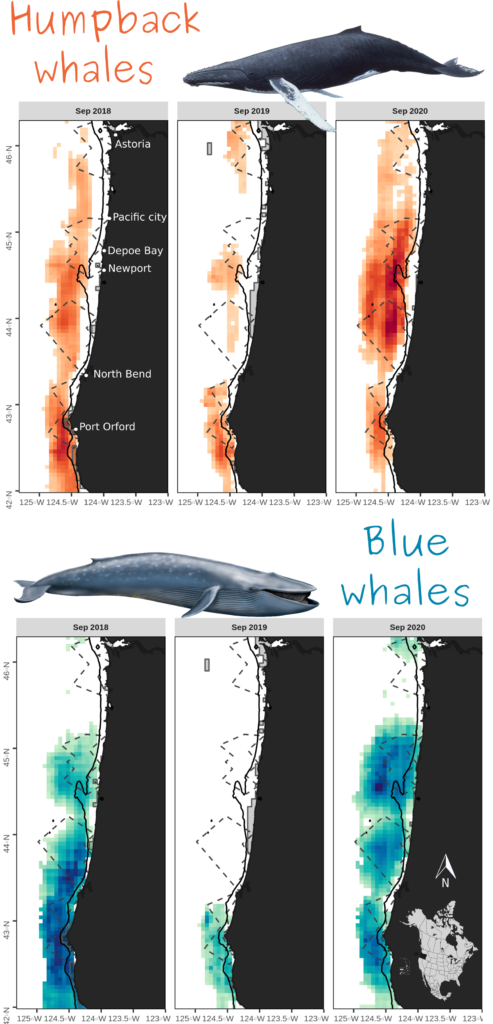
Across multiple cross-validations of the species-specific models, sea surface temperature, sea surface height and depth were recurrently selected among the most important variables influencing both humpback and blue whale distributions. Predicted densities of blue whales were relatively higher at less than 40 fathoms compared to humpback whales, although both species’ hotspots were located outside this newly implemented seasonal fishing limit (Figure 2). Higher densities were generally predicted off Newport and Port Orford, and north of North Bend.

Figure 2: Predicted densities of humpback and blue whales during the month of September 2018, 2019, and 2020 in Oregon waters (OPAL project). Core areas of use (predicted densities in the top 25%) are represented, with darker shades of blue and orange showing higher predicted densities. Dashed lines represent the tracklines followed by USCG monthly aerial surveys. The black line represents the 40 fathom isobath. Grey boxes overlayed on predictions delineate the areas of extrapolation where environmental conditions are non-analogous to the conditions in which the models were trained. Disclaimer: these model outputs are preliminary and should be interpreted with caution.

Once our rorqual models are finalized, we will work with our partners at the Oregon Department of Fisheries and Wildlife to overlay predicted whale hotspots with areas of high crab pot densities. This overlap analysis will help us understand the times and places where co-occurrence of suitable whale habitat and fishing activities put whales at risk of entanglement.

References

Archer, F. I., Morin, P. A., Hancock-Hanser, B. L., Robertson, K. M., Leslie, M. S., Bérubé, M., … Taylor, B. L. (2013). Mitogenomic Phylogenetics of Fin Whales (Balaenoptera physalus spp.): Genetic Evidence for Revision of Subspecies. PLoS ONE, 8(5). https://doi.org/10.1371/journal.pone.0063396

Becker, E. A., Forney, K. A., Redfern, J. V, Barlow, J., Jacox, M. G., Roberts, J. J., & Palacios, D. M. (2019). Predicting cetacean abundance and distribution in a changing climate. Diversity and Distributions, 25(4), 626–643. https://doi.org/10.1111/ddi.12867

Fleming, A. H., Clark, C. T., Calambokidis, J., & Barlow, J. (2016). Humpback whale diets respond to variance in ocean climate and ecosystem conditions in the California Current. Global Change Biology, 22, 1214–1224. https://doi.org/10.1111/gcb.13171

Fossette, S., Abrahms, B., Hazen, E. L., Bograd, S. J., Zilliacus, K. M., Calambokidis, J., … Croll, D. A. (2017). Resource partitioning facilitates coexistence in sympatric cetaceans in the California Current. Ecology and Evolution, 7, 9085–9097. https://doi.org/10.1002/ece3.3409

Jefferson, T. A., Palacios, D. M., Clambokidis, J., Baker, S. C., Hayslip, C. E., Jones, P. A., … Schulman-Janiger, A. (2021). Sightings and Satellite Tracking of a Blue / Fin Whale Hybrid in its Wintering and Summering Ranges in the Eastern North Pacific. Advances in Oceanography & Marine Biology, 2(4), 1–9. https://doi.org/10.33552/AOMB.2021.02.000545

Jefferson, T. A., Webber, M. A., & Pitman, R. L. (2008). Marine Mammals of the World. A comprehensive guide to their identification. Elsevier, London, UK.

Mizroch, S. A., Rice, D. W., Zwiefelhofer, D., Waite, J., & Perryman, W. L. (2009). Distribution and movements of fin whales in the North Pacific Ocean. Mammal Review, 39(3), 193–227. https://doi.org/10.1111/j.1365-2907.2009.00147.x

NOAA Fisheries. (2018). Fin whale stock assessment report ( Balaenoptera physalus physalus ): California / Oregon / Washington Stock.

Scales, K. L., Schorr, G. S., Hazen, E. L., Bograd, S. J., Miller, P. I., Andrews, R. D., … Falcone, E. A. (2017). Should I stay or should I go? Modelling year-round habitat suitability and drivers of residency for fin whales in the California Current. Diversity and Distributions, 23(10), 1204–1215. https://doi.org/10.1111/ddi.12611

Making predictions: A window into ecological forecast models

By Dawn Barlow, PhD Candidate, OSU Department of Fisheries, Wildlife and Conservation Sciences, Geospatial Ecology of Marine Megafauna Lab

“What is the weather going to be like tomorrow?” “How long will it take to drive there, with traffic?” We all rely on forecasts to make decisions, such as whether to bring a rain jacket, when to get in the car to arrive at a certain destination on time, or any number of situations where we want a prediction of what will happen in the near future. Statistical models underpin many of these examples, using past data to inform future predictions.

Early on in graduate school, I was told that “all models are wrong, but some models work.” Any model is essentially a best approximation, using mathematical relationships, of how we understand a pattern. Models are powerful tools in ecology, enabling us to distill complex, dynamic, and interacting systems into terms and parameters that can be quantified. This ability can help us better understand our study systems and use that understanding to make predictions. We will never be able to describe every nuance of an ecosystem. Instead, the challenge is to collect enough information to build an informed model that can enhance our understanding, without over-simplifying or unnecessarily complicating the system we aim to describe. As Dr. Simon Levin stated in his 1989 seminal paper:

A good model does not attempt to reproduce every detail of the biological system; the system itself suffices for that purpose as the most detailed model of itself. Rather, the objective of a model should be to ask how much detail can be ignored without producing results that contradict specific sets of observations, on particular scales of interest.”1

Species distribution models (SDMs) are the particular branch of models that underpin much of my PhD research on blue whale ecology and distribution in New Zealand. SDMs are mathematical algorithms that correlate observations of a species with environmental conditions at their observed locations to gain ecological insight and predict spatial distributions of the species (Fig. 1)2. The model is a best attempt to quantify and describe the relationships between predictors, e.g., temperature and the observed species distribution pattern. For example, blue whale occurrence is higher in areas of lower temperatures and greater krill availability, and these relationships can be described with models3. So, a model essentially takes all the data available, and synthesizes that information in terms of the relationships between the predictors (environment) and response (species occurrence). Then, we can look at the fitted relationships to ask what we would expect from the species distribution pattern when temperature, or krill availability, or any other predictor, is at a particular value. 

Figure 1. A schematic of a species distribution model (SDM) illustrating how the relationship between mapped species and environmental data (left) is compared to describe “environmental space” (center), and then map predictions from a model using only environmental predictors (right). Note that inter-site distances in geographic space might be quite different from those in environmental space—a and c are close geographically, but not environmentally. The patterning in the predictions reflects the spatial autocorrelation of the environmental predictors. Figure reproduced from Elith and Leathwick (2009).

So, if a model is simply a mathematical description of how terms interact to produce a particular outcome, how do predictions work? To make a spatial prediction, e.g., a map of the probability of a species being present, you need two things: a model describing the functional relationships between species presence and your environmental predictors, and the values of your predictor variables on the day you are interested in predicting to. For example, you may need to obtain a map of sea surface temperature, productivity, temperature anomaly, and surface currents on a day you want to know where whales are expected to be. Your model is the applied across that stack of spatial environmental layers and, based on the functional relationships derived by the model, you get an estimate of the probability of species occurrence based on the temperature, productivity, anomaly, and surface current values at each location. By applying the model over a range of values, you can obtain a continuous surface with the probability of presence, in the form of a map. These maps are typically for the past or present because that is when we can typically acquire spatial environmental layers. However, to make predictions for a future time of interest, we need to have spatial environmental layers for the future.

Forecasts are predictions for the future. Recent advances in technology and computing have led to an emergence of environmental and ecological forecasting tools that are being developed around the world to produce marine forecasts. These tools include predictions of the physical environment such as ocean temperatures or currents, and biological patterns such as where species will be distributed in space and timing of events like salmon spawning or lobster landings4. The ability to generate forecast of marine ecosystems is of particular interest to resource users and managers because it can allow them to be proactive rather than reactive. Forecasts enable us to anticipate events or patterns and prepare, rather than having to respond in real-time or after the fact.

The South Taranaki Bight region in New Zealand is an area where blue whale foraging habitat frequently coincides with industry pressures, including petroleum and mineral extraction, exploration for petroleum reserves using seismic airgun surveys, vessel traffic between ports, and even an ongoing proposal for seabed mining5. Static spatial restrictions to mitigate impacts from these activities on blue whales may be met with resistance from industry user groups, but dynamic spatial management6–8 of blue whale habitat could be more attractive and acceptable. The key for successful dynamic management is knowing where and when to put those boundaries; and this is where ecological forecast models can show their strength. If we can predict suitable blue whale habitat for the future, proactive regulations can be applied to enhance conservation management in the region. Can we develop reliable and useful ecological forecasts for the South Taranaki Bight? Well, given that we have already developed robust models of the relationships between blue whales and their habitat3 and have documented the spatial and temporal lags between wind, upwelling, and blue whales9, we feel confident that we can develop forecast models to predict where blue whales will be in the STB region. As we continue working hard toward this goal, we invite you to check back for our findings in the future. So, consider this blog post a forecast of sorts, and stay tuned!  

Figure 2. A blue whale surfaces in front of an oil extraction platform in the South Taranaki Bight, demonstrating the overlap between whales and industry in the region. Photo by D. Elvines.

References:

1.        Levin, S. A. The problem of pattern and scale. Ecology 73, 1943–1967 (1992).

2.        Elith, J. & Leathwick, J. R. Species Distribution Models: Ecological Explanation and Prediction Across Space and Time. Annu. Rev. Ecol. Evol. Syst. 40, 677–697 (2009).

3.        Barlow, D. R., Bernard, K. S., Escobar-Flores, P., Palacios, D. M. & Torres, L. G. Links in the trophic chain: Modeling functional relationships between in situ oceanography, krill, and blue whale distribution under different oceanographic regimes. Mar. Ecol. Prog. Ser. 642, 207–225 (2020).

4.        Payne, M. R. et al. Lessons from the first generation of marine ecological forecast products. Front. Mar. Sci. 4, 1–15 (2017).

5.        Torres, L. G. Evidence for an unrecognised blue whale foraging ground in New Zealand. New Zeal. J. Mar. Freshw. Res. 47, 235–248 (2013).

6.        Hyrenbach, K. D., Forney, K. A. & Dayton, P. K. Marine protected areas and ocean basin management. Aquat. Conserv. Mar. Freshw. Ecosyst. 10, 437–458 (2000).

7.        Maxwell, S. M. et al. Dynamic ocean management: Defining and conceptualizing real-time management of the ocean. Mar. Policy 58, 42–50 (2015).

8.        Oestreich, W. K., Chapman, M. S. & Crowder, L. B. A comparative analysis of dynamic management in marine and terrestrial systems. Front. Ecol. Environ. 18, 496–504 (2020).

9.        Barlow, D. R., Klinck, H., Ponirakis, D., Garvey, C. & Torres, L. G. Temporal and spatial lags between wind, coastal upwelling, and blue whale occurrence. Sci. Rep. 11, (2021).

Inference, and the intersection of ecology and statistics

By Dawn Barlow, PhD student, OSU Department of Fisheries and Wildlife, Geospatial Ecology of Marine Megafauna Lab

Recently, I had the opportunity to attend the International Statistical Ecology Conference (ISEC), a biennial meeting of researchers at the interface of ecology and statistics. I am a marine ecologist, fascinated by the interactions between animals and the dynamic ocean environment they inhabit. If you had asked me five years ago whether I thought I would ever consider myself a statistician or a computer programmer, my answer would certainly have been “no”. Now, I find myself studying the ecology of blue whales in New Zealand using a variety of data streams and methodologies, but a central theme for my dissertation is species distribution modeling. Species distribution models (SDMs) are mathematical algorithms that correlate observations of a species with environmental conditions at their observed locations to gain ecological insight and predict spatial distributions of the species (Fig. 1; Elith and Leathwick 2009). I still can’t say I would identify as a statistician, but I have a growing appreciation for the role of statistics to gain inference in ecology.

Figure 1. A schematic of a species distribution model (SDM) illustrating how the relationship between mapped species and environmental data (left) is compared to describe “environmental space” (center), and then map predictions from a model using only environmental predictors (right). Note that inter-site distances in geographic space might be quite different from those in environmental space—a and c are close geographically, but not environmentally. The patterning in the predictions reflects the spatial autocorrelation of the environmental predictors. Figure reproduced from Elith and Leathwick (2009).

Before I continue, let’s take a look at just a few definitions from Merriam-Webster’s dictionary:

Statistics: a branch of mathematics dealing with the collection, analysis, interpretation, and presentation of masses of numerical data

Ecology: a branch of science concerned with the interrelationship of organisms and their environments

Inference: a conclusion or opinion that is formed because of known facts or evidence

Ecological data are notoriously noisy, messy, and complex. Statistical tests are meant to help us understand whether a pattern in the data is different from what we would expect through random chance. When we study how organisms interact with one another and their environment, it is impossible to completely capture all elements of the ecosystem. Therefore, ecology is a field ripe with challenges for statisticians. How do we quantify a meaningful biological signal amidst all the noise? How can we gain inference from ecological data to enhance knowledge, and how can we use that knowledge to make informed predictions? Marine mammals are notoriously difficult to study. They inhabit an environment that is relatively inaccessible and inhospitable to humans, they occur in low numbers, they are highly mobile, and they are rarely visible. All ecological data are difficult and noisy and riddled with small sample sizes, but counting trees presents fewer logistical challenges than counting moving whales in an ever-changing open-ocean setting. Therefore, new methodologies in areas like species distribution modeling are often developed using large, terrestrial datasets and eventually migrate to applications in the marine environment (Robinson et al. 2011).

Many presentations I attended at the conference were geared toward moving beyond correlative SDMs. SDMs were developed to correlate species occurrence patterns with features of the environment they inhabit (e.g. temperature, precipitation, terrain, etc.). However, those relationships do not actually explain the underlying mechanism of why a species is more likely to occur in one environment compared to another. Therefore, ecological statisticians are now using additional information and modeling approaches within SDMs to incorporate information such as species co-occurrence patterns, population demographic information, and physiological constraints. Building SDMs to include such process-explicit information allows us to make steps toward understanding not just when and where a species occurs, but why.

Machine learning is an area that continues to advance and open doors to new applications in ecology. Machine learning approaches differ fundamentally from classical statistics. In statistics, we formulate a hypothesis, select the appropriate model to test that hypothesis (for example, linear regression), then test how well the data fit the model (“Is the relationship linear?”), and test the strength of that inference (“Is the linear pattern different from what we would expect due to random chance?”). Machine learning, on the other hand, does not use a predetermined notion of relationships between variables. Rather, it tries to create an algorithm that fits the patterns in the data. Statistics asks how well the data fit a model, and machine learning asks how well a model fits the data.

Machine learning approaches allow for very complex relationships to be included in models and can be excellent for making predictions. However, sometimes the relationships fitted by a machine learning algorithm are so complex that it is not possible to infer any ecological meaning from them. As one ISEC presenter put it, in machine learning “the computer learns but the scientist does not”. The most important thing when selecting your methodology is to remember your question and your goal. Do you want to understand the mechanism of why an animal is where it is? Or do you not need to understand the driver, but rather want to make the best predictions of where an animal will be? In my case, the answer to that question differs from one of my PhD chapters to the next. We want to understand the functional relationships between oceanography, krill availability, and blue whale distribution (Barlow et al. 2020), and subsequently we want to develop forecasting models that can reliably predict blue whale distribution to inform conservation efforts (Fig. 2).

Figure 2. An example predictive map of where we expect blue whales to be distributed based on environmental conditions. Warmer colors represent areas with a higher probability of blue whale occurrence, and the blue crosses represent locations where blue whales were observed.

ISEC was an excellent opportunity for me to break out of my usual marine mammal-centered bubble and get a taste of what is happening on the leading edge of statistical ecology. I learned about the latest approaches and innovations in species distribution modeling, and in the process I also learned about trees, koalas, birds, and many other organisms from around the world. A fun bonus of attending a methods-focused conference is learning about completely new study species and systems. There are many ways of approaching an ecological question, gaining inference, and making predictions. I look forward to incorporating the knowledge I gained through ISEC into my own research, both in my doctoral work and in applications of new methods to future research projects.

Figure 3. The virtual conference photo of all who attended the biennial International Statistical Ecology Conference. Thank you to the organizers, who made it a truly excellent and engaging conference experience!

References

Barlow, D.R., Bernard, K.S., Escobar-Flores, P., Palacios, D.M., and Torres, L.G. 2020. Links in the trophic chain: Modeling functional relationships between in situ oceanography, krill, and blue whale distribution under different oceanographic regimes. Mar. Ecol. Prog. Ser. doi:https://doi.org/10.3354/meps13339.

Elith, J., and Leathwick, J.R. 2009. Species Distribution Models: Ecological Explanation and Prediction Across Space and Time. Annu. Rev. Ecol. Evol. Syst. 40(1): 677–697. doi:10.1146/annurev.ecolsys.110308.120159.

Robinson, L.M., Elith, J., Hobday, A.J., Pearson, R.G., Kendall, B.E., Possingham, H.P., and Richardson, A.J. 2011. Pushing the limits in marine species distribution modelling: Lessons from the land present challenges and opportunities. doi:10.1111/j.1466-8238.2010.00636.x.

The teamwork of conservation science

Dr. Leigh Torres
PI, Geospatial Ecology of Marine Megafauna Lab, Marine Mammal Institute
Assistant Professor, Oregon Sea Grant, Department of Fisheries and Wildlife, Oregon State University

I have played on sports teams all my life – since I was four until present day. Mostly soccer teams, but a fair bit of Ultimate too. Teams are an interesting beast. They can be frustrating when communication breaks down, irritating when everyone is not on the same timeline, and disastrous if individuals do not complete their designated job. Yet, without the whole team we would never win. So, on top of the fun of competition, skill development, and exercise, playing on teams has always been part of the challenging and fulfilling process for me: everyone working toward the same goal – to win – by making the team fluid, complimentary, integrated, and ultimately successful.

I have come to learn that it is the same with conservation science.

A few of my teams through the ages, as player and coach. Some of my favorite people are on these teams, from 1981 to 2018.

Conservation efforts are often so complex, that it is practically impossible to achieve success alone. Forces driving the need for conservation typically include monetary needs/desires, social values, ecological processes, animal physiology, multi-jurisdictional policies, and human behavior. Each one of these forces alone is challenging to understand and takes expertise to comprehend the situation. Hence, building a well-functioning team is essential. Here’s a recent example from the GEMM Lab:

Since 2014 entanglements of blue, humpback and gray whales in fishing gear along the west coast of the USA have dramatically increased, particularly in Dungeness crab fishing gear. Many forces likely led to this increase, including increased whale population abundance, potential shifts in whale distributions, and changes in fishing fleet dynamics. While we cannot point a finger at one cause, many people and groups recognize that we cannot continue to let whales become entangled and killed at such high rates: whale populations would decline, fisheries would look bad in the public eye and potentially lose profits, whales have an intrinsic right to live in the ocean without being bycaught, and whales are an important part of the ecosystem that would deteriorate without them. In 2017, the Oregon Whale Entanglement Working Group was formed to bring stakeholders together that were concerned about this problem to discuss possible solutions and paths forward. I was lucky to be a part of this group, which also included members of the Dungeness crab fishery and commission, the Oregon Department of Fish and Wildlife (ODFW), other marine mammal scientists, and representatives of the American Cetacean Society, The Nature Conservancy, and a local marine gear supplier.

We met regularly over 2.5 years, and despite some hesitation at first about walking into a room of potentially disgruntled fishermen (I would be lying if I did not admit to this), after the first meeting I looked forward to every gathering. I learned an immense amount about the Dungeness crab fishery and how it operates, how ODFW manages the fishery and why, and what people do, don’t and need to know about whales in Oregon. Everyone agreed that reducing whale entanglements is needed, and a frequent approach discussed was to reduce risk by not setting gear where and when we expect whales to be. Yet, this idea flagged a very critical knowledge gap: We do not have a good understanding of whale distribution patterns in Oregon. Thus leading to the development of a highly collaborative research effort to describe whale distribution patterns in Oregon and identify areas of co-occurrence between whales and fishing effort to reduce the risk of entanglements. Sounds great, but a tough task to accomplish in a few short years. So, let me introduce the great team I am working with to make it all happen.

While I may know a few things about whales and spatial ecology, I don’t know too much about fisheries in Oregon. My collaboration with folks at ODFW, particularly Kelly Corbett and Troy Buell, has enabled this project to develop and go forward, and ultimately will lead to success. These partners provide feedback about how and where the fishery operates so I know where and when to collect data, and importantly they will provide the information on fishing effort in Oregon waters to relate to our generated maps of whale distribution. This spatial comparison will produce what is needed by managers and fishermen to make informed and effective decisions about where to fish, and not to fish, so that we reduce whale entanglement risk while still harvesting successfully to ensure the health and sustainability of our coastal economies.

So, how can we collect standardized data on whale distribution in Oregon waters without breaking the bank? I tossed this question around for a long time, and then I looked up to the sky and wondered what that US Coast Guard (USCG) helicopter was flying around for all the time. I reached out to the USCG to enquire, and proposed that we have an observer fly in the helicopter with them along a set trackline during their training flights. Turns out the USCG Sector North Bend and Columbia River were eager to work with us and support our research. They have turned out to be truly excellent partners in this work. We had some kinks to work out at the beginning – lots of acronyms, protocols, and logistics for both sides to figure out – but everyone has been supportive and pleasant to work with. The pilots and crew are interested in our work and it is a joy to hear their questions and see them learn about the marine ecosystem. And our knowledge of helicopter navigation and USCG duties has grown astronomically.

On the left is a plot of the four tracklines we survey for whales each month for two years aboard a US Coast Guard helicopter. On the right are some photos of us in action with our Coast Guard partners.

Despite significant cost savings to the project through our partnership with the USCG, we still need funds to support time, gear and more. And full credit to the Oregon Dungeness Crab Commission for recognizing the value and need for this project to support their industry, and stepping up to fund the first year of this project. Without their trust and support the project may not have got off the ground. With this support in our back pocket and proof of our capability, ODFW and I teamed up to approach the National Oceanographic and Atmospheric and Administration (NOAA) for funds to support the remaining years of the project. We found success through the NOAA Fisheries Endangered Species Act Section 6 Program, and we are now working toward providing the information needed to protect endangered and threatened whales in Oregon waters.

Despite our cost-effective and solid approach to data collection on whale occurrence, we cannot be everywhere all the time looking for whales. So we have also teamed up with Amanda Gladics at Oregon Sea Grant to help us with an important outreach and citizen science component of the project. With Amanda we have developed brochures and videos to inform mariners of all kinds about the project, objectives, and need for them to play a part. We are encouraging everyone to use the Whale Alert app to record their opportunistic sightings of whales in Oregon waters. These data will help us build and test our predictive models of whale distribution. Through this partnership we continue important conversations with fishermen from many fisheries about their concerns, where they are seeing whales, and what needs to be done to solve this complex conservation challenge.  

Of course I cannot collect, process, analyze, and interpret all this data on my own. I do not have the skills or capacity for that. My partner in the sky is Craig Hayslip, a Faculty Research Assistant in the Marine Mammal Institute. Craig has immense field experience collecting data on whales and is the primary observer on the survey flights. Together we have navigated the USCG world and developed methods to collect our data effectively and efficiently (all within a tiny space flying over the ocean). In a few months we will be ¾ of the way through our data collection phase, which means data analysis will take over. For this phase I am bringing back a GEMM Lab star, Solene Derville, who recently completed her PhD. As the post-doc on the project, Solene will take the lead on the species distribution modeling and fisheries overlap analysis. I am looking forward to partnering with Solene again to compile multiple data sources on whales and oceanography in Oregon to produce reliable and accurate predictions of whale occurrence and entanglement risk. Finally I want to acknowledge our great partners at the Cascadia Research Collective (Olympia, WA) and the Cetacean Conservation and Genomics Lab (OSU, Marine Mammal Institute) who help facilitate our data collection, and conduct the whale photo-identification or genetic analyses to determine population assignment.  

As you can see, even this one, smallish, conservation research project takes a diverse team of partners to proceed and ensure success. On this team, my position is sometimes a player, coach, or manager, but I am always grateful for these amazing collaborations and opportunities to learn. I am confident in our success and will report back on our accomplishments as we wrap up this important and exciting conservation science project.   

A fin whale observed off the Oregon coast during one of our surveys aboard a US Coast Guard helicopter.

Species distribution modeling: Part statistics, part philosophy, and there is no “right answer”

By Dawn Barlow, PhD student, OSU Department of Fisheries and Wildlife, Geospatial Ecology of Marine Megafauna Lab

Just like that, I have wrapped up year 1 of my PhD in Wildlife Science. For my PhD, I am investigating the ecology and distribution of blue whales in New Zealand across multiple spatial and temporal scales. In a region where blue whales overlap with industrial activity, there is considerable interest from managers to be able to reliably forecast when and where blue whales are most likely to be in the area. In a series of five chapters and utilizing multiple different data sources (dedicated boat surveys, oceanographic data, acoustic recordings, remotely sensed environmental data, opportunistic blue whale sightings information), I will attempt to describe, quantify, and predict where blue whales are found in relation to their environment. Each chapter will evaluate the distribution of blue whales relative to the environment at different scales in space (ranging from 4 km to 25 km resolution) and time (ranging from daily to seasonal resolution). One overarching method I am using throughout my PhD is species distribution modeling. Having just completed my research review with my doctoral committee last week, I’ll share this aspect of my research proposal that I’ve particularly enjoyed reading, writing, and thinking about.

A pair of blue whales surfacing in the South Taranaki Bight region of New Zealand. Drone piloted by Todd Chandler during the 2017 field season.

Species distribution models (SDMs), which are sometimes referred to as habitat models or ecological niche models, are mathematical algorithms that combine observations of a species with environmental conditions at their observed locations, to gain ecological insight and predict spatial distributions of the species (Elith and Leathwick, 2009; Redfern et al., 2006). Any model is just one description of what is occurring in the natural world. Just as there are many ways to describe something with words and many languages to do so, there are many options for modeling frameworks and approaches, with stark and nuanced differences. My labmate and friend Solene Derville has equated the number of choices one has for SDMs to the cracker section in an American grocery store. When navigating all of these choices and considerations, it is important to remember that no model will ever be completely correct—it is our best attempt at describing a complex natural system—and as an analyst we need to do the best that we can with the data available to address the ecological questions at hand. As it turns out, the dividing line between quantitative analysis and philosophy is thin at times. What may seem at first like a purely objective, statistical endeavor requires careful consideration and fundamental decision-making on the part of the analyst.

Ecosystems are multifaceted, complex, and hierarchical. They are comprised of multiple physical and biological components, which operate at multiple scales across space and time. As Dr. Simon Levin stated in at 1989 MacArthur Award lecture on the topic of scale in ecology:

“A good model does not attempt to reproduce every detail of the biological system; the system itself suffices for that purpose as the most detailed model of itself. Rather, the objective of a model should be to ask how much detail can be ignored without producing results that contradict specific sets of observations, on particular scales of interest” (Levin, 1992).

The question of scale is central to ecology. As many biology students learn in their first introductory classes, parsimony is “The principle that the most acceptable explanation of an occurrence, phenomenon, or event is the simplest, involving the fewest entities, assumptions, or changes” (Oxford Dictionary). In other words, the best explanation is the simplest one. One challenge in ecological modeling, including SDMs, is to select spatial and temporal scales as coarse as possible for the most parsimonious—the most straightforward—model, while still being fine enough to capture relevant patterns. Another critical consideration is the scale of the question you are interested in answering. The scale of the analysis must match the scale at which you want to make inferences about the ecology of a species.

Similarly, the issue of complexity is central to distribution modeling. Overly simple models may not be able to adequately describe the relationship between species occurrence and the environment. In contrast, highly complex models may have very high explanatory power, but risk ascribing an ecological pattern to noise in the data (Merow et al., 2014), in other words, finding patterns that aren’t real. Furthermore, highly complex models tend to have poorer predictive capacity than simpler models (Merow et al., 2014). There is a trade-off between descriptive and predictive power in SDMs (Derville et al., 2018). Therefore, a key component in the SDM process is establishing the end goal of the model with respect to the region of interest, scale, explanatory power, predictive capacity, and in many cases management need.

Finally, any model is ultimately limited by the data available and the scale at which it was collected (Elith and Leathwick, 2009; Guillera-Arroita et al., 2015; Redfern et al., 2006). Prior knowledge of what environmental features are important to the species of interest is often limited at the time of the data collection effort, and data collection is constrained by when it is logistically feasible to sample. For example, we collect detailed oceanographic data during the summer months when it is practical to get out on the water, satellite imagery of sea surface temperature might be unavailable during times of cloud cover, and people are more likely to report blue whale sightings in areas where there is more human activity. Therefore, useful SDMs that address both ecological and management needs typically balance the scale of analysis and model complexity with the limitations of the data.

Managers and politicians within the New Zealand government are interested in a tool to predict when and where blue whales are most likely to be, based on sound ecological analysis. This is one of the end-goals of my PhD, but in the meantime, I am grappling with the appropriate scales of analysis, and attempting to balance questions of model complexity, explanatory power, and predictive capacity. There is no single, correct answer, and so my process is in part quantitative analysis, part philosophy, and all with the goal of increased ecological understanding and conservation of a species.

A blue whale breaks the surface. As I grapple with questions of model complexity and scale of analysis, I sometimes need a reminder that behind each data point is a blue whale, and what a privilege it is to study them. Photo by Leigh Torres.

References:

Derville, S., Torres, L. G., Iovan, C., and Garrigue, C. (2018). Finding the right fit: Comparative cetacean distribution models using multiple data sources and statistical approaches. Divers. Distrib. 24, 1657–1673. doi:10.1111/ddi.12782.

Elith, J., and Leathwick, J. R. (2009). Species Distribution Models: Ecological Explanation and Prediction Across Space and Time. Annu. Rev. Ecol. Evol. Syst. 40, 677–697. doi:10.1146/annurev.ecolsys.110308.120159.

Guillera-Arroita, G., Lahoz-Monfort, J. J., Elith, J., Gordon, A., Kujala, H., Lentini, P. E., et al. (2015). Is my species distribution model fit for purpose? Matching data and models to applications. Glob. Ecol. Biogeogr. 24, 276–292. doi:10.1111/geb.12268.

Levin, S. A. (1992). The problem of pattern and scale. Ecology 73, 1943–1967.

Merow, C., Smith, M. J., Edwards, T. C., Guisan, A., Mcmahon, S. M., Normand, S., et al. (2014). What do we gain from simplicity versus complexity in species distribution models? Ecography (Cop.). 37, 1267–1281. doi:10.1111/ecog.00845.

Redfern, J. V., Ferguson, M. C., Becker, E. A., Hyrenbach, K. D., Good, C., Barlow, J., et al. (2006). Techniques for cetacean-habitat modeling. Mar. Ecol. Prog. Ser. 310, 271–295. doi:10.3354/meps310271.

Zooming in: A closer look at bottlenose dolphin distribution patterns off of San Diego, CA

By: Alexa Kownacki, Ph.D. Student, OSU Department of Fisheries and Wildlife, Geospatial Ecology of Marine Megafauna Lab

Data analysis is often about parsing down data into manageable subsets. My project, which spans 34 years and six study sites along the California coast, requires significant data wrangling before full analysis. As part of a data analysis trial, I first refined my dataset to only the San Diego survey location. I chose this dataset for its standardization and large sample size; the bulk of my sightings, over 4,000 of the 6,136, are from the San Diego survey site where the transect methods were highly standardized. In the next step, I selected explanatory variable datasets that covered the sighting data at similar spatial and temporal resolutions. This small endeavor in analyzing my data was the first big leap into understanding what questions are feasible in terms of variable selection and analysis methods. I developed four major hypotheses for this San Diego site.

The study species: common bottlenose dolphin (Tursiops truncatus) seen along the California coastline in 2015. Image source: Alexa Kownacki.

Hypotheses:

H1: I predict that bottlenose dolphin sightings along the San Diego transect throughout the years 1981-2015 exhibit clustered distribution patterns as a result of the patchy distributions of both the species’ preferred habitats, as well as the social nature of bottlenose dolphins.

H2: I predict there would be higher densities of bottlenose dolphin at higher latitudes spanning 1981-2015 due to prey distributions shifting northward and less human activities in the northerly sections of the transect.

H3: I predict that during warm (positive) El Niño Southern Oscillation (ENSO) months, the dolphin sightings in San Diego would be distributed more northerly, predominantly with prey aggregations historically shifting northward into cooler waters, due to (secondarily) increasing sea surface temperatures.

H4: I predict that along the San Diego coastline, bottlenose dolphin sightings are clustered within two kilometers of the six major lagoons, with no specific preference for any lagoon, because the murky, nutrient-rich waters in the estuarine environments are ideal for prey protection and known for their higher densities of schooling fishes.

Data Description:

The common bottlenose dolphin (Tursiops truncatus) sighting data spans 1981-2015 with a few gap years. Sightings cover all months, but not in all years sampled. The same transect in San Diego was surveyed in a small, rigid-hulled inflatable boat with approximately a two-kilometer observation area (one kilometer surveyed 90 degrees to starboard and port of the bow).

I wanted to see if there were changes in dolphin distribution by latitude and, if so, whether those changes had a relationship to ENSO cycles and/or distances to lagoons. For ENSO data, I used the NOAA database that provides positive, neutral, and negative indices (1, 0, and -1, respectively) by each month of each year. I matched these ENSO data to my month-date information of dolphin sighting data. Distance from each lagoon was calculated for each sighting.

Figure 1. Map representing the San Diego transect, represented with a light blue line inside of a one-kilometer buffered “sighting zone” in pale yellow. The dark pink shapes are dolphin sightings from 1981-2015, although some are stacked on each other and cannot be differentiated. The lagoons, ranging in size, are color-coded. The transect line runs from the breakwaters of Mission Bay, CA to Oceanside Harbor, CA.

Results: 

H1: True, dolphins are clustered and do not have a uniform distribution across this area. Spatial analysis indicated a less than a 1% likelihood that this clustered pattern could be the result of random chance (Fig. 1, z-score = -127.16, p-value < 0.0001). It is well-known that schooling fishes have a patchy distribution, which could influence the clustered distribution of their dolphin predators. In addition, bottlenose dolphins are highly social and although pods change in composition of individuals, the dolphins do usually transit, feed, and socialize in small groups.

Figure 2. Summary from the Average Nearest Neighbor calculation in ArcMap 10.6 displaying that bottlenose dolphin sightings in San Diego are highly clustered. When the z-score, which corresponds to different colors on the graphic above, is strongly negative (< -2.58), in this case dark blue, it indicates clustering. Because the p-value is very small, in this case, much less than 0.01, these results of clustering are strongly significant.

H2: False, dolphins do not occur at higher densities in the higher latitudes of the San Diego study site. The sightings are more clumped towards the lower latitudes overall (p < 2e-16), possibly due to habitat preference. The sightings are closer to beaches with higher human densities and human-related activities near Mission Bay, CA. It should be noted, that just north of the San Diego transect is the Camp Pendleton Marine Base, which conducts frequent military exercises and could deter animals.

Figure 3. Histogram comparing the latitudes with the frequency of dolphin sightings in San Diego, CA. The x-axis represents the latitudinal difference from the most northern part of the transect to each dolphin sighting. Therefore, a small difference would translate to a sighting being in the northern transect areas whereas large differences would translate to sightings being more southerly. This could be read from left to right as most northern to most southern. The y-axis represents the frequency of which those differences are seen, that is, the number of sightings with that amount of latitudinal difference, or essentially location on the transect line. Therefore, you can see there is a peak in the number of sightings towards the southern part of the transect line.

H3: False, during warm (positive) El Niño Southern Oscillation (ENSO) months, the dolphin sightings in San Diego were more southerly. In colder (negative) ENSO months, the dolphins were more northerly. The differences between sighting latitude and ENSO index was significant (p<0.005). Post-hoc analysis indicates that the north-south distribution of dolphin sightings was different during each ENSO state.

Figure 4. Boxplot visualizing distributions of dolphin sightings latitudinal differences and ENSO index, with -1,0, and 1 representing cold, neutral, and warm years, respectively.

H4: True, dolphins are clustered around particular lagoons. Figure 5 illustrates how dolphin sightings nearest to Lagoon 6 (the San Dieguito Lagoon) are always within 0.03 decimal degrees. Because of how these data are formatted, decimal degrees is the easiest way to measure change in distance (in this case, the difference in latitude). In comparison, dolphins at Lagoon 5 (Los Penasquitos Lagoon) are distributed across distances, with the most sightings further from the lagoon.

Figure 5. Bar plot displaying the different distances from dolphin sighting location to the nearest lagoon in San Diego in decimal degrees. Note: Lagoon 4 is south of the study site and therefore was never the nearest lagoon.

I found a significant difference between distance to nearest lagoon in different ENSO index categories (p < 2.55e-9): there is a significant difference in distance to nearest lagoon between neutral and negative values and positive and neutral years. Therefore, I hypothesize that in neutral ENSO months compared to positive and negative ENSO months, prey distributions are changing. This is one possible hypothesis for the significant difference in lagoon preference based on the monthly ENSO index. Using a violin plot (Fig. 6), it appears that Lagoon 5, Los Penasquitos Lagoon, has the widest variation of sighting distances in all ENSO index conditions. In neutral years, Lagoon 0, the Buena Vista Lagoon has multiple sightings, when in positive and negative years it had either no sightings or a single sighting. The Buena Vista Lagoon is the most northerly lagoon, which may indicate that in neutral ENSO months, dolphin pods are more northerly in their distribution.

Figure 6. Violin plot illustrating the distance from lagoons of dolphin sightings under different ENSO conditions. There are three major groups based on ENSO index: “-1” representing cold years, “0” representing neutral years, and “1” representing warm years. On the x-axis are lagoon IDs and on the y-axis is the distance to the nearest lagoon in decimal degrees. The wider the shapes, the more sightings, therefore Lagoon 6 has many sightings within a very small distance compared to Lagoon 5 where sightings are widely dispersed at greater distances.


Bottlenose dolphins foraging in a small group along the California coast in 2015. Image source: Alexa Kownacki.

Takeaways to science and management: 

Bottlenose dolphins have a clustered distribution which seems to be related to ENSO monthly indices, and likely, their social structures. From these data, neutral ENSO months appear to have something different happening compared to positive and negative months, that is impacting the sighting distributions of bottlenose dolphins off the San Diego coastline. More research needs to be conducted to determine what is different about neutral months and how this may impact this dolphin population. On a finer scale, the six lagoons in San Diego appear to have a spatial relationship with dolphin sightings. These lagoons may provide critical habitat for bottlenose dolphins and/or for their preferred prey either by protecting the animals or by providing nutrients. Different lagoons may have different spans of impact, that is, some lagoons may have wider outflows that create larger nutrient plumes.

Other than the Marine Mammal Protection Act and small protected zones, there are no safeguards in place for these dolphins, whose population hovers around 500 individuals. Therefore, specific coastal areas surrounding lagoons that are more vulnerable to habitat loss, habitat degradation, and/or are more frequented by dolphins, may want greater protection added at a local, state, or federal level. For example, the Batiquitos and San Dieguito Lagoons already contain some Marine Conservation Areas with No-Take Zones within their reach. The city of San Diego and the state of California need better ways to assess the coastlines in their jurisdictions and how protecting the marine, estuarine, and terrestrial environments near and encompassing the coastlines impacts the greater ecosystem.

This dive into my data was an excellent lesson in spatial scaling with regards to parsing down my data to a single study site and in matching my existing data sets to other data that could help answer my hypotheses. Originally, I underestimated the robustness of my data. At first, I hesitated when considering reducing the dolphin sighting data to only include San Diego because I was concerned that I would not be able to do the statistical analyses. However, these concerns were unfounded. My results are strongly significant and provide great insight into my questions about my data. Now, I can further apply these preliminary results and explore both finer and broader scale resolutions, such as using the more precise ENSO index values and finding ways to compare offshore bottlenose dolphin sighting distributions.

Data Wrangling to Assess Data Availability: A Data Detective at Work

By Alexa Kownacki, Ph.D. Student, OSU Department of Fisheries and Wildlife, Geospatial Ecology of Marine Megafauna Lab

Data wrangling, in my own loose definition, is the necessary combination of both data selection and data collection. Wrangling your data requires accessing then assessing your data. Data collection is just what it sounds like: gathering all data points necessary for your project. Data selection is the process of cleaning and trimming data for final analyses; it is a whole new bag of worms that requires decision-making and critical thinking. During this process of data wrangling, I discovered there are two major avenues to obtain data: 1) you collect it, which frequently requires an exorbitant amount of time in the field, in the lab, and/or behind a computer, or 2) other people have already collected it, and through collaboration you put it to a good use (often a different use then its initial intent). The latter approach may result in the collection of so much data that you must decide which data should be included to answer your hypotheses. This process of data wrangling is the hurdle I am facing at this moment. I feel like I am a data detective.

Data wrangling illustrated by members of the R-programming community. (Image source: R-bloggers.com)

My project focuses on assessing the health conditions of the two ecotypes of bottlenose dolphins between the waters off of Ensenada, Baja California, Mexico to San Francisco, California, USA between 1981-2015. During the government shutdown, much of my data was inaccessible, seeing as it was in possession of my collaborators at federal agencies. However, now that the shutdown is over, my data is flowing in, and my questions are piling up. I can now begin to look at where these animals have been sighted over the past decades, which ecotypes have higher contaminant levels in their blubber, which animals have higher stress levels and if these are related to geospatial location, where animals are more susceptible to human disturbance, if sex plays a role in stress or contaminant load levels, which environmental variables influence stress levels and contaminant levels, and more!

Alexa, alongside collaborators, photographing transiting bottlenose dolphins along the coastline near Santa Barbara, CA in 2015 as part of the data collection process. (Image source: Nick Kellar).

Over the last two weeks, I was emailed three separate Excel spreadsheets representing three datasets, that contain partially overlapping data. If Microsoft Access is foreign to you, I would compare this dilemma to a very confusing exam question of “matching the word with the definition”, except with the words being in different languages from the definitions. If you have used Microsoft Access databases, you probably know the system of querying and matching data in different databases. Well, imagine trying to do this with Excel spreadsheets because the databases are not linked. Now you can see why I need to take a data management course and start using platforms other than Excel to manage my data.

A visual interpretation of trying to combine datasets being like matching the English definition to the Spanish translation. (Image source: Enchanted Learning)

In the first dataset, there are 6,136 sightings of Common bottlenose dolphins (Tursiops truncatus) documented in my study area. Some years have no sightings, some years have fewer than 100 sightings, and other years have over 500 sightings. In another dataset, there are 398 bottlenose dolphin biopsy samples collected between the years of 1992-2016 in a genetics database that can provide the sex of the animal. The final dataset contains records of 774 bottlenose dolphin biopsy samples collected between 1993-2018 that could be tested for hormone and/or contaminant levels. Some of these samples have identification numbers that can be matched to the other dataset. Within these cross-reference matches there are conflicting data in terms of amount of tissue remaining for analyses. Sorting these conflicts out will involve more digging from my end and additional communication with collaborators: data wrangling at its best. Circling back to what I mentioned in the beginning of this post, this data was collected by other people over decades and the collection methods were not standardized for my project. I benefit from years of data collection by other scientists and I am grateful for all of their hard work. However, now my hard work begins.

The cutest part of data wrangling: finding adorable images of bottlenose dolphins, photographed during a coastal survey. (Image source: Alexa Kownacki).

There is also a large amount of data that I downloaded from federally-maintained websites. For example, dolphin sighting data from research cruises are available for public access from the OBIS (Ocean Biogeographic Information System) Sea Map website. It boasts 5,927,551 records from 1,096 data sets containing information on 711 species with the help of 410 collaborators. This website is incredible as it allows you to search through different data criteria and then download the data in a variety of formats and contains an interactive map of the data. You can explore this at your leisure, but I want to point out the sheer amount of data. In my case, the OBIS Sea Map website is only one major platform that contains many sources of data that has already been collected, not specifically for me or my project, but will be utilized. As a follow-up to using data collected by other scientists, it is critical to give credit where credit is due. One of the benefits of using this website, is there is information about how to properly credit the collaborators when downloading data. See below for an example:

Example citation for a dataset (Dataset ID: 1201):

Lockhart, G.G., DiGiovanni Jr., R.A., DePerte, A.M. 2014. Virginia and Maryland Sea Turtle Research and Conservation Initiative Aerial Survey Sightings, May 2011 through July 2013. Downloaded from OBIS-SEAMAP (http://seamap.env.duke.edu/dataset/1201) on xxxx-xx-xx.

Citation for OBIS-SEAMAP:

Halpin, P.N., A.J. Read, E. Fujioka, B.D. Best, B. Donnelly, L.J. Hazen, C. Kot, K. Urian, E. LaBrecque, A. Dimatteo, J. Cleary, C. Good, L.B. Crowder, and K.D. Hyrenbach. 2009. OBIS-SEAMAP: The world data center for marine mammal, sea bird, and sea turtle distributions. Oceanography 22(2):104-115

Another federally-maintained data source that boasts more data than I can quantify is the well-known ERDDAP website. After a few Google searches, I finally discovered that the acronym stands for Environmental Research Division’s Data Access Program. Essentially, this the holy grail of environmental data for marine scientists. I have downloaded so much data from this website that Excel cannot open the csv files. Here is yet another reason why young scientists, like myself, need to transition out of using Excel and into data management systems that are developed to handle large-scale datasets. Everything from daily sea surface temperatures collected on every, one-degree of latitude and longitude line from 1981-2015 over my entire study site to Ekman transport levels taken every six hours on every longitudinal degree line over my study area. I will add some environmental variables in species distribution models to see which account for the largest amount of variability in my data. The next step in data selection begins with statistics. It is important to find if there are highly correlated environmental factors prior to modeling data. Learn more about fitting cetacean data to models here.

The ERDAPP website combined all of the average Sea Surface Temperatures collected daily from 1981-2018 over my study site into a graphical display of monthly composites. (Image Source: ERDDAP)

As you can imagine, this amount of data from many sources and collaborators is equal parts daunting and exhilarating. Before I even begin the process of determining the spatial and temporal spread of dolphin sightings data, I have to identify which data points have sex identified from either hormone levels or genetics, which data points have contaminants levels already quantified, which samples still have tissue available for additional testing, and so on. Once I have cleaned up the datasets, I will import the data into the R programming package. Then I can visualize my data in plots, charts, and graphs; this will help me identify outliers and potential challenges with my data, and, hopefully, start to see answers to my focal questions. Only then, can I dive into the deep and exciting waters of species distribution modeling and more advanced statistical analyses. This is data wrangling and I am the data detective.

What people may think a ‘data detective’ looks like, when, in reality, it is a person sitting at a computer. (Image source: Elder Research)

Like the well-known phrase, “With great power comes great responsibility”, I believe that with great data, comes great responsibility, because data is power. It is up to me as the scientist to decide which data is most powerful at answering my questions.

Data is information. Information is knowledge. Knowledge is power. (Image source: thedatachick.com)


Finding the right fit: a journey into cetacean distribution models

Solène Derville, Entropie Lab, French National Institute for Sustainable Development (IRD – UMR Entropie), Nouméa, New Caledonia

 Ph.D. student under the co-supervision of Dr. Leigh Torres

Species Distribution Models (SDM), also referred to as ecological niche models, may be defined as “a model that relates species distribution data (occurrence or abundance at known locations) with information on the environmental and/or spatial characteristics of those locations” (Elith & Leathwick, 2009)⁠. In the last couple decades, SDMs have become an indispensable part of the ecologists’ and conservationists’ toolbox. What scientist has not dreamed of being able to summarize a species’ environmental requirements and predict where and when it will occur, all in one tiny statistical model? It sounds like magic… but the short acronym “SDM” is the pretty front window of an intricate and gigantic research field that may extend way beyond the skills of a typical ecologist (even so for a graduate student like myself).

As part of my PhD thesis about the spatial ecology of humpback whales in New Caledonia, South Pacific, I was planning on producing a model to predict their distribution in the region and help spatial planning within the Natural Park of the Coral Sea. An innocent and seemingly perfectly feasible plan for a second year PhD student. To conduct this task, I had at my disposal more than 1,000 sightings recorded during dedicated surveys at sea conducted over 14 years. These numbers seem quite sufficient, considering the rarity of cetaceans and the technical challenges of studying them at sea. And there was more! The NGO Opération Cétacés  also recorded over 600 sightings reported by the general public in the same time period and deployed more than 40 satellite tracking tags to follow individual whale movements. In a field where it is so hard to acquire data, it felt like I had to use it all, though I was not sure how to combine all these types of data, with their respective biases, scales and assumptions.

One important thing about SDM to remember: it is like a cracker section in a US grocery shop, there is sooooo much choice! As I reviewed the possibilities and tested various modeling approaches on my data I realized that this study might be a good opportunity to contribute to the SDM field, by conducting a comparison of various algorithms using cetacean occurrence data from multiple sources. The results of this work was just published  in Diversity and Distributions:

Derville S, Torres LG, Iovan C, Garrigue C. (2018) Finding the right fit: Comparative cetacean distribution models using multiple data sources and statistical approaches. Divers Distrib. 2018;00:1–17. https://doi. org/10.1111/ddi.12782

There are simply too many! Anonymous grocery shops, Corvallis, OR
Credit: Dawn Barlow

If you are a new-comer to the SDM world, and specifically its application to the marine environment, I hope you find this interesting. If you are a seasoned SDM user, I would be very grateful to read your thoughts in the comment section! Feel free to disagree!

So what is the take-home message from this work?

  • There is no such thing as a “best model”; it all depends on what you want your model to be good at (the descriptive vs predictive dichotomy), and what criteria you use to define the quality of your models.

The predictive vs descriptive goal of the model: This is a tricky choice to make, yet it should be clearly identified upfront. Most times, I feel like we want our models to be decently good at both tasks… It is a risky approach to blindly follow the predictions of a complex model without questioning the meaning of the ecological relationships it fitted. On the other hand, conservation applications of models often require the production of predicted maps of species’ probability of presence or habitat suitability.

The criteria for model selection: How could we imagine that the complexity of animal behavior could be summarized in a single metric, such as the famous Akaike Information criterion (AIC) or the Area under the ROC Curve (AUC)? My study, and that of others (e.g. Elith & Graham  H., 2009),⁠ emphasize the importance of looking at multiple aspects of model outputs: raw performance through various evaluation metrics (e.g. see AUCdiff; (Warren & Seifert, 2010)⁠, contribution of the variables to the model, shape of the fitted relationships through Partial Dependence Plots (PDP, Friedman, 2001),⁠ and maps of predicted habitat suitability and associated error. Spread all these lines of evidence in front of you, summarize all the metrics, add a touch of critical ecological thinking to decide on the best approach for your modeling question, and Abracadabra! You end up a bit lost in a pile of folders… But at least you assessed the quality of your work from every angle!

  • Cetacean SDMs often serve a conservation goal. Hence, their capacity to predict to areas / times that were not recorded in the data (which is often scarce) is paramount. This extrapolation performance may be restricted when the model relationships are overfitted, which is when you made your model fit the data so closely that you are unknowingly modeling noise rather than a real trend. Using cross-validation is a good method to prevent overfitting from happening (for a thorough review: Roberts et al., 2017)⁠. Also, my study underlines that certain algorithms inherently have a tendency to overfit. We found that Generalized Additive Models and MAXENT provided a valuable complexity trade-off to promote the best predictive performance, while minimizing overfitting. In the case of GAMs, I would like to point out the excellent documentation that exist on their use (Wood, 2017)⁠, and specifically their application to cetacean spatial ecology (Mannocci, Roberts, Miller, & Halpin, 2017; Miller, Burt, Rexstad, & Thomas, 2013; Redfern et al., 2017).⁠
  • Citizen science is a promising tool to describe cetacean habitat. Indeed, we found that models of habitat suitability based on citizen science largely converged with those based on our research surveys. The main issue encountered when modeling this type of data is the absence of “effort”. Basically, we know where people observed whales, but we do not know where they haven’t… or at least not with the accuracy obtained from research survey data. However, with some information about our citizen scientists and a little deduction, there is actually a lot you can infer about opportunistic data. For instance, in New Caledonia most of the sightings were reported by professional whale-watching operators or by the general public during fishing/diving/boating day trips. Hence, citizen scientists rarely stray far from harbors and spend most of their time in the sheltered waters of the New Caledonian lagoon. This reasoning provides the sort of information that we integrated in our modeling approach to account for spatial sampling bias of citizen science data and improve the model’s predictive performance.

Many more technical aspects of SDM are brushed over in this paper (for detailed and annotated R codes of the modeling approaches, see supplementary information of our paper). There are a few that are not central to the paper, but that I think are worth sharing:

  • Collinearity of predictors: Have you ever found that the significance of your predictors completely changed every time you removed a variable? I have progressively come to discover how unstable a model can be because of predictor collinearity (and the uneasy feeling that comes with it …). My new motto is to ALWAYS check cross-correlation between my predictors, and do it THOROUGHLY. A few aspects that may make a big difference in the estimation of collinearity patterns are to: (1) calculate Pearson vs Spearman coefficients, (2) check correlations between the values recorded at the presence points vs over the whole study area, and (3) assess the correlations between raw environmental variables vs between transformed variables (log-transformed, etc). Though selecting variables with Pearson coefficients < 0.7 is usually a good rule (Dormann et al., 2013), I would worry of anything above 0.5, or at least keep it in mind during model interpretation.
  • Cross-validation: If removing 10% of my dataset greatly impacts the model results, I feel like cross-validation is critical. The concept is based on a simple assumption, if I had sampled a given population/phenomenon/system slightly differently, would I have come to the same conclusion? Cross-validation comes in many different methods, but the basic concept is to run the same model several times (number of times may depend on the size of your data set, hierarchical structure of your data, computation power of your computer, etc.) over different chunks of your data. Model performance metrics (e.g., AUC) and outputs (e.g., partial dependence plots) are than summarized on the many runs, using mean/median and standard deviation/quantiles. It is up to you how to pick these chunks, but before doing this at random I highly recommend reading Roberts et al. (2017).

The evil of the R2: I am probably not the first student to feel like what I have learned in my statistical classes at school is in practice, at best, not very useful, and at worst, dangerously misleading. Of course, I do understand that we must start somewhere, and that learning the basics of inferential statistics is a necessary step to, one day, be able to answer your one research questions. Yet, I feel like I have been carrying the “weight of the R2” for far too long before actually realizing that this metric of model performance (R2 among others) is simply not  enough to trust my results. You might think that your model is robust because among the 1000 alternative models you tested, it is the one with the “best” performance (deviance explained, AIC, you name it), but the model with the best R2 will not always be the most ecologically meaningful one, or the most practical for spatial management perspectives. Overfitting is like a sword of Damocles hanging over you every time you create a statistical model All together, I sometimes trust my supervisor’s expertise and my own judgment more than an R2.

Source: internet

A few good websites/presentations that have helped me through my SDM journey:

General website about spatial analysis (including SDM): http://rspatial.org/index.html

Cool presentation by Adam Smith about SDM:

http://www.earthskysea.org/!ecology/sdmShortCourseKState2012/sdmShortCourse_kState.pdf

Handling spatial data in R: http://www.maths.lancs.ac.uk/~rowlings/Teaching/UseR2012/introductionTalk.html

“The magical world of mgcv”, a great presentation by Noam Ross: https://www.youtube.com/watch?v=q4_t8jXcQgc


Literature cited

Dormann, C. F., Elith, J., Bacher, S., Buchmann, C., Carl, G., Carré, G., … Lautenbach, S. (2013). Collinearity: A review of methods to deal with it and a simulation study evaluating their performance. Ecography, 36(1), 027–046. https://doi.org/10.1111/j.1600-0587.2012.07348.x

Elith, J., & Graham  H., C. (2009). Do they? How do they? WHY do they differ? On finding reasons for differing performances of species distribution models . Ecography, 32(Table 1), 66–77. https://doi.org/10.1111/j.1600-0587.2008.05505.x

Elith, J., & Leathwick, J. R. (2009). Species Distribution Models: Ecological Explanation and Prediction Across Space and Time. Annual Review of Ecology, Evolution, and Systematics, 40(1), 677–697. https://doi.org/10.1146/annurev.ecolsys.110308.120159

Friedman, J. H. (2001). Greedy Function Approximation: A gradient boosting machine. The Annals of Statistics, 29(5), 1189–1232. Retrieved from http://www.jstor.org/stable/2699986

Mannocci, L., Roberts, J. J., Miller, D. L., & Halpin, P. N. (2017). Extrapolating cetacean densities to quantitatively assess human impacts on populations in the high seas. Conservation Biology, 31(3), 601–614. https://doi.org/10.1111/cobi.12856.This

Miller, D. L., Burt, M. L., Rexstad, E. A., & Thomas, L. (2013). Spatial models for distance sampling data: Recent developments and future directions. Methods in Ecology and Evolution, 4(11), 1001–1010. https://doi.org/10.1111/2041-210X.12105

Redfern, J. V., Moore, T. J., Fiedler, P. C., de Vos, A., Brownell, R. L., Forney, K. A., … Ballance, L. T. (2017). Predicting cetacean distributions in data-poor marine ecosystems. Diversity and Distributions, 23(4), 394–408. https://doi.org/10.1111/ddi.12537

Roberts, D. R., Bahn, V., Ciuti, S., Boyce, M. S., Elith, J., Guillera-Arroita, G., … Dormann, C. F. (2017). Cross-validation strategies for data with temporal, spatial, hierarchical or phylogenetic structure. Ecography, 0, 1–17. https://doi.org/10.1111/ecog.02881

Warren, D. L., & Seifert, S. N. (2010). Ecological niche modeling in Maxent: the importance of model complexity and the performance of model selection criteria. Ecological Applications, 21(2), 335–342. https://doi.org/10.1890/10-1171.1

Wood, S. N. (2017). Generalized additive models: an introduction with R (second edi). CRC press.