Clicks, buzzes, and rasps: How the MMPA has spurred what we know about beaked whale acoustic repertoire

By Marissa Garcia, PhD Student, Cornell University, Department of Natural Resources and the Environment, K. Lisa Yang Center for Conservation Bioacoustics

In October 1972, the tides turned for U.S. environmental politics: the Marine Mammal Protection Act (MMPA) was passed. Its creation ushered in a new flavor of conservation and management. With phrases like “optimum sustainable population” baked into its statutory language, it marked among the first times that ecosystem-based management — an approach which directly calls upon knowledge of ecology to inform action — was required by law (Ray and Potter 2022). Transitioning from reductionist, species-siloed policies, the MMPA instead placed the interdependency of species at the core of ecosystem function and management. 

Beyond deepening the role of science on Capitol Hill, the MMPA’s greatest influence may have been spurred by the language that prohibited “the taking and importation of marine mammals” (16 U.S.C. 1361). Because the word “taking” is multivalent, it carries on its back many interpretations. “Taking” a marine mammal is not limited to intentionally hunting or killing them, or even accidental bycatch. “Taking” also includes carelessly operating a boat when a marine mammal is present, feeding a marine mammal in the wild, or tagging a marine mammal without the appropriate scientific permit. “Taking” a marine mammal can also extend to the fatal consequences caused by noise pollution — not intent, but incident (16 U.S.C. 1362).

The latter circumstances remain reverberant for the U.S. Navy. To comply with the MMPA, they are granted “incidental, but not intentional, taking of small numbers of marine mammals….[when] engag[ing] in a specified activity (other than commercial fishing)” (87 FR 33113). So, if the sonar activities required for national security exercises adversely impact marine mammals, the Navy has a bit of leeway but is still expected to minimize this impact. To further mitigate this potential harm, the Navy thus invests heavily in marine mammal research. (If you are interested in learning more about how the Navy has influenced the trajectory of oceanographic research more broadly, you may find this book interesting.) 

Beaked whales are an example of a marine mammal we know much about due to the MMPA’s call for research when incidental take occurs. Three decades ago, many beaked whales stranded ashore following a series of U.S. Navy sonar exercises. Since then, the Navy has flooded research dollars toward better understanding beaked whale hearing, vocal behavior, and movements (e.g., Klinck et al. 2012). Through these efforts, a deluge of research charged with developing effective tools to acoustically monitor and conserve beaked whales has emerged.  

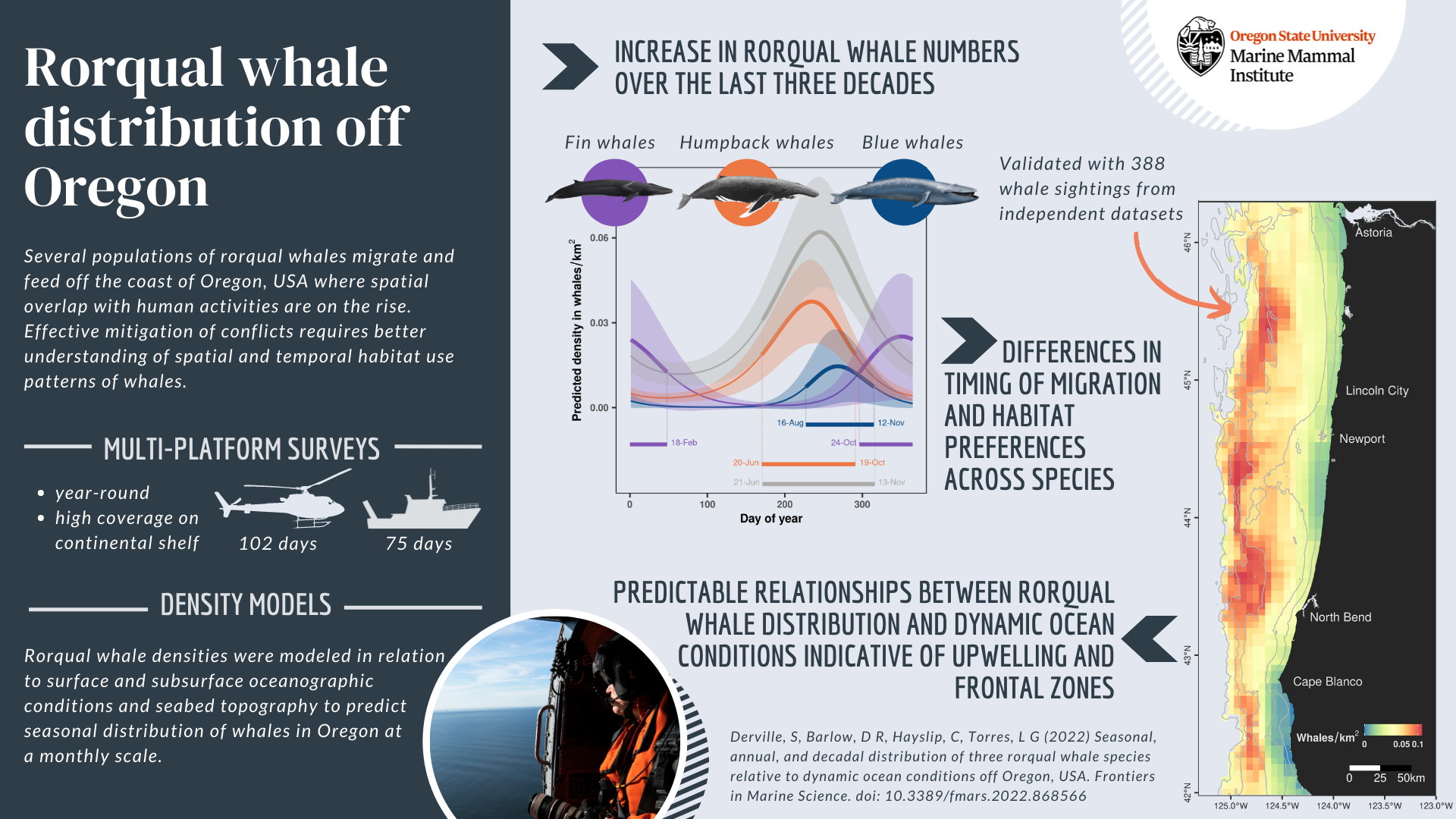
These studies have laid the foundation for my Ph.D. research, which is dedicated to the Holistic Assessment of Living marine resources off Oregon (HALO) project. Through both visual and acoustic surveys, the HALO project’s mission is to understand how changes in ocean conditions — driven by global climate change — influence living marine resources in Oregon waters. 

In my research specifically, I aim to learn more about beaked whales off the Oregon coast. Beaked whales represent nearly a fourth of cetacean species alive today, with at least 21 species recorded to date (Roman et al. 2013). Even so, 90% of beaked whales are considered data deficient: we lack enough information about them to confidently describe the state of their populations or decide upon effective conservation action. 

Much remains to be learned about beaked whales, and I aim to do so by eavesdropping on them. By referring to the “acoustic repertoire” of beaked whales — that is, their vocalizations and corresponding behaviors — I aim to tease out their vocalizations from the broader ocean soundscape and understand how their presence in Oregon waters varies over time. 

Beaked whales are notoriously cryptic, elusive to many visual survey efforts like those aboard HALO cruises. In fact, some species have only been identified via carcasses that have washed ashore (Moore and Barlow 2013). Acoustic studies have elucidated ecological information (beaked whales forage at night at seamounts summits; Johnston et al. 2008) and have also introduced promising population-level monitoring efforts (beaked whales have been acoustically detected in areas with a historical scarcity of sightings; Kowarski et al. 2018). Their deep-diving nature often renders them inconspicuous, and they forage at depths between 1,000 and 2,000 m, on dives as long as 90 minutes (Moore and Barlow 2013; Klinck et al. 2012). Their echolocation clicks are produced at frequencies within the hearing range of killer whales, and previous studies have suggested that Blainville’s beaked whales are only vocally active during deep foraging dives and not at the surface, possibly to prevent being acoustically detected by predatory killer whales. Researchers refer to this phenomenon as “acoustic crypsis,” or when vocally-active marine mammals are strategically silent to avoid being found by potential predators (Aguilar de Soto et al. 2012).

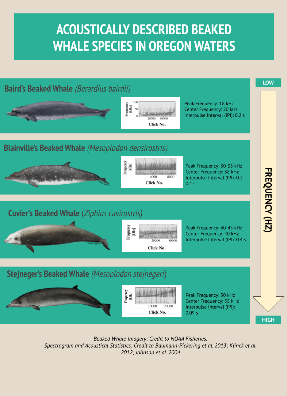
We expect to see evidence of Blainville’s beaked whales in Oregon waters, as well as Baird’s, Cuvier’s, Stejneger’s, Hubb’s, and other beaked whale species. Species-specific echolocation clicks were comprehensively described a decade ago in Baumann-Pickering et al. 2013 (Figure 1). While this study laid the groundwork for species-level beaked whale acoustic detection, much more work is still needed to describe their acoustic repertoire with higher resolution detail. For example, though Hubb’s beaked whales live in Oregon waters, their vocal behavior remains scantly defined.

Figure 1: Baird’s, Blainville’s, Cuvier’s, and Stejneger’s beaked whales are among the most comprehensively acoustically described beaked whales inhabiting central Oregon waters, though more work would improve accuracy in species-specific acoustic detection. Credit: Marissa Garcia. Infographic draws upon beaked whale imagery from NOAA Fisheries and spectrograms and acoustical statistics published in Baumann-Pickering et al. 2013.

The HALO project seeks to add a biological dimension to the historical oceanographic studies conducted along the Newport Hydrographic (NH) line ever since the 1960s (Figure 2). Rockhopper acoustic recording units are deployed at sites NH 25, NH 45, and NH 65. The Rockhopper located at site NH 65 is actively recording on the seafloor about 2,800 m below the surface. Because beaked whales tend to be most vocally active at these deep depths, we will first dive into the acoustic data on NH 65, our deepest unit, in hopes of finding beaked whale recordings there.

Figure 2: The HALO project team conducts quarterly visual surveys along the NH line, spanning between NH 25 and NH 65. Rockhopper acoustic recording units continuously record at the NH 25, NH 45, and NH 65 sites. Credit: Leigh Torres.

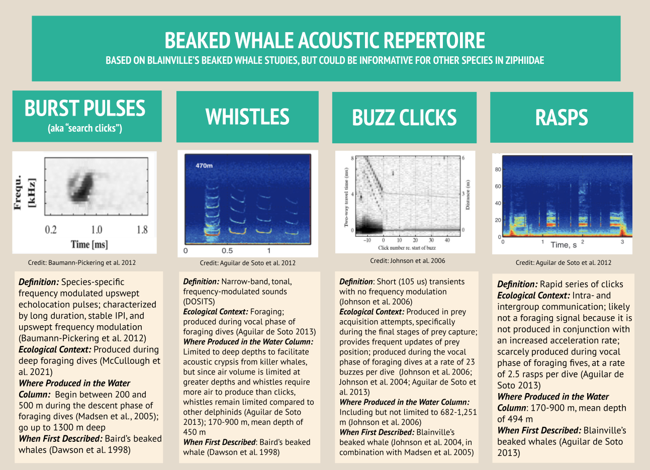
Beaked whales’ acoustic repertoire can be broadly split into four primary categories: burst pulses (aka “search clicks”), whistles, buzz clicks, and rasps. Beaked whale search clicks, which are regarded as burst pulses when produced in succession, have distinct qualities: their upswept frequency modulation (meaning the frequency gets higher within the click), their long duration especially when compared to other delphinid clicks, and a consistent interpulse interval  which is the time of silence between signals (Baumann-Pickering et al. 2013). Acoustic analysts can identify different species based on how the frequency changes in different burst pulse sequences (Baumann-Pickering et al. 2013; Figure 1). For this reason, when I conduct my HALO analyses, I intend to automatically detect beaked whale species using burst pulses, as they are the best documented beaked whale signal, with unique signatures for each species. 

In the landscape of beaked whale acoustics, the acoustic repertoire of Blainville’s beaked whales (Mesoplodon densirostris) — a species of focus in my HALO analyses — is especially well defined. Blainville’s beaked whale whistles have been recorded up to 900 m deep, representing the deepest whistle recorded for any marine mammal to date in the literature (Aguilar de Soto et al. 2012). While Blainville’s beaked whales only spend 40% of their time at depths below 170 m, two key vocalizations occur at these depths: whistles and rasps. While they remain surprisingly silent near the surface, beaked whales produce whistles and rasps at depths up to 900 m. The beaked whales dive together in synchrony, and right before they separate from each other, they produce the most whistles and rasps, further indicating that these vocalizations are used to enhance foraging success (Aguilar de Soto et al. 2006). As beaked whales transition to foraging on their own, they predominantly produce frequently modulated clicks and buzzes. Beaked whales produce buzzes in the final stages of prey capture to receive up-to-date information about their prey’s location. The buzzes’ high repetition enables the whale to achieve 300+ updates on their intended prey’s location in the last 3 m before seizing their feast (Johnson et al. 2006; Figure 3). 

Figure 3: Blainville’s beaked whales generally have four categories within their acoustic repertoire, including burst pulses, whistles, buzz clicks, and rasps. Credit: Marissa Garcia.

All of this knowledge about beaked whale acoustics can be linked back to the MMPA, which has also achieved broader success. Since the MMPA’s implementation, marine mammal population numbers have risen across the board. For marine mammal populations with sufficient data, approximately 65% of these stocks are increasing and 17% are stable (Roman et al. 2013). 

Nevertheless, perhaps much of the MMPA’s true success lies in the research it has indirectly fueled, by virtue of the required compliance of governmental bodies such as the U.S. Navy. And the response has proven to be a boon to knowledge: if the U.S. Navy has been the benefactor of marine mammal research, beaked whale acoustics has certainly been the beneficiary. We hope the beaked whale acoustic analyses stemming from the HALO Project can further this expanse of what we know.

Loading

References

Aguilar de Soto, N., Madsen, P. T., Tyack, P., Arranz, P., Marrero, J., Fais, A., Revelli, E., & Johnson, M. (2012). No shallow talk: Cryptic strategy in the vocal communication of Blainville’s beaked whales. Marine Mammal Science, 28(2), E75–E92. https://doi.org/10.1111/j.1748-7692.2011.00495.x

Baumann-Pickering, S., McDonald, M. A., Simonis, A. E., Solsona Berga, A., Merkens, K. P. B., Oleson, E. M., Roch, M. A., Wiggins, S. M., Rankin, S., Yack, T. M., & Hildebrand, J. A. (2013). Species-specific beaked whale echolocation signals. The Journal of the Acoustical Society of America, 134(3), 2293–2301. https://doi.org/10.1121/1.4817832

Dawson, S., Barlow, J., & Ljungblad, D. (1998). SOUNDS RECORDED FROM BAIRD’S BEAKED WHALE, BERARDIUS BAIRDIL. Marine Mammal Science, 14(2), 335–344. https://doi.org/10.1111/j.1748-7692.1998.tb00724.x

Johnston, D. W., McDonald, M., Polovina, J., Domokos, R., Wiggins, S., & Hildebrand, J. (2008). Temporal patterns in the acoustic signals of beaked whales at Cross Seamount. Biology Letters (2005), 4(2), 208–211. https://doi.org/10.1098/rsbl.2007.0614

Johnson, M., Madsen, P. T., Zimmer, W. M. X., de Soto, N. A., & Tyack, P. L. (2004). Beaked whales echolocate on prey. Proceedings of the Royal Society. B, Biological Sciences, 271(Suppl 6), S383–S386. https://doi.org/10.1098/rsbl.2004.0208

Johnson, M., Madsen, P. T., Zimmer, W. M. X., de Soto, N. A., & Tyack, P. L. (2006). Foraging Blainville’s beaked whales (Mesoplodon densirostris) produce distinct click types matched to different phases of echolocation. Journal of Experimental Biology, 209(Pt 24), 5038–5050. https://doi.org/10.1242/jeb.02596

Klinck, H., Mellinger, D. K., Klinck, K., Bogue, N. M., Luby, J. C., Jump, W. A., Shilling, G. B., Litchendorf, T., Wood, A. S., Schorr, G. S., & Baird, R. W. (2012). Near-real-time acoustic monitoring of beaked whales and other cetaceans using a Seaglider. PloS One, 7(5), e36128. https://doi.org/10.1371/annotation/57ad0b82-87c4-472d-b90b-b9c6f84947f8

Kowarski, K., Delarue, J., Martin, B., O’Brien, J., Meade, R., Ó Cadhla, O., & Berrow, S. (2018). Signals from the deep: Spatial and temporal acoustic occurrence of beaked whales off western Ireland. PloS One, 13(6), e0199431–e0199431. https://doi.org/10.1371/journal.pone.0199431

Madsen, P. T.,  Johnson, M., de Soto, N. A., Zimmer, W. M. X., & Tyack, P. (2005). Biosonar performance of foraging beaked whales (Mesoplodon densirostris). Journal of Experimental Biology, 208(Pt 2), 181–194. https://doi.org/10.1242/jeb.01327

McCullough, J. L. K., Wren, J. L. K., Oleson, E. M., Allen, A. N., Siders, Z. A., & Norris, E. S. (2021). An Acoustic Survey of Beaked Whales and Kogia spp. in the Mariana Archipelago Using Drifting Recorders. Frontiers in Marine Science, 8. https://doi.org/10.3389/fmars.2021.664292

Moore, J. E. & Barlow, J. P. (2013). Declining abundance of beaked whales (family Ziphiidae) in the California Current large marine ecosystem. PloS One, 8(1), e52770–e52770. https://doi.org/10.1371/journal.pone.0052770

Ray, G. C. & Potter, F. M. (2011). The Making of the Marine Mammal Protection Act of 1972. Aquatic Mammals, 37(4), 522.

Roman, J., Altman, I., Dunphy-Daly, M. M., Campbell, C., Jasny, M., & Read, A. J. (2013). The Marine Mammal Protection Act at 40: status, recovery, and future of U.S. marine mammals. Annals of the New York Academy of Sciences, 1286(1), 29–49. https://doi.org/10.1111/nyas.12040

Marine Science Pride: The Significance of Representation in the Workplace

Morgan O’Rourke-Liggett, Graduate Student, OSU Department of Fisheries, Wildlife, and Conservation Sciences, Geospatial Ecology of Marine Megafauna Lab

October is LGBTQIA2S+ (Lesbian, Gay, Bisexual, Transgender, Intersex, Asexual, Aromatic, Agender, Two-Spirit, plus) History Month in the United States. As a marine biologist and member of the LGBTQIA2S+ community, I publicly came out in 2016. Since then, I have been navigating coming out in the workplace. As a graduate student, I’m using this time to practice being an “out” marine biologist.

OutInSTEM, a student organization at Oregon State University (OSU), supports LGBTQIA2S+ students in science, technology, engineering, and mathematics (STEM). It provides mentorship and connection with faculty and other students in the LGBTQIA2S+ community. Another goal is to increase visibility in the profession and foster confidence in students as they continue their professional careers. Other initiatives like OutInSTEM exist in many forms across agencies and countries.

Within the National Oceanographic and Atmospheric Administration (NOAA), the National Marine Sanctuary System created the initiative #PrideInTheOcean to celebrate both Ocean Month and LGBTQIA2S+ Pride Month, which both occur in June in the United States. This program partners with Pride Outside, a group connecting the LGBTQIA2S+ community through outdoor activities.

Some notable LGBTQIA2S+ scientists in marine studies are members and alumni of the Marine Mammal Institute at OSU. One is Dominique Kone (He/Him) who is now a marine ecologist and science officer at the California Ocean Science Trust. He is a graduate of OSU’s Marine Mammal Institute and the GEMM laboratory. Dominique wrote about his story here on Ocean Wise. Another is Dr. Daniel Palacios (He/Him), Endowed Associate Professor in Whale Habitats and lead of the Whale Habitat, Ecology, and Telemetry laboratory (WHET Lab) at OSU’s Marine Mammal Institute. Read Daniel’s story here on 500 Queer Scientists.

Visibility and representation are critical for multiple reasons. One is creating an atmosphere where LGBTQIA2S+ members feel validated in their experiences, allowing them to express their opinions, and recognize their contributions. Without the stress of facing potential harassment in the workplace, we can be our genuine selves leading to a healthier work environment, increased engagement, and better results.

Not everyone can be “out” in all aspects of their life. Some may be out publicly, but not at work; only out to select friends, etc. If it’s not safe (financially, physically, etc.), some people are never able to come out. Personal safety usually drives this decision. Some don’t want to expose aspects of their personal life in the workplace. Others hide it until after they have been hired or passed the probation period. Some never share due to fear of reprisal, such as being passed over for a promotion.

Despite the presence of state and federal anti-discrimination policies, micro and macro-aggressions occur in the workplace, such as transgender people having to fight for appropriate housing assignments. As a fisheries biological technician in Alaska, I was moved around several times as they had never dealt with a non-binary, transmasculine professional in their dorm rooms. I was forced to move three times and was frequently misgendered and deadnamed (deadnaming is calling a transgender person by an incorrect name, often their birth name and no longer use upon transitioning). It was a difficult situation and negatively affected my personal and work experience. I felt demoralized, disheartened, and depressed. I lost my respect for the agency and my long-standing dream of working in Alaska. 

To avoid repeating my experience in Alaska, perhaps we can think critically about our labs and workspaces. The following is a non-exhaustive list of things to consider when including and thinking about LGBTQIA2S+ co-workers:

  • How are transgender and other gender-diverse co-workers treated?
  • Does your place of work have gender-inclusive restrooms on every floor of the building?
  • Are dorms or berths separated by binary gender?
  • Do the men’s restrooms have menstruation products and baby changing station(s)?
  • Does your field gear include sizing options for people who have non-conforming bodies?
  • If your lab does events including significant others, is the environment welcoming of same-gender spouses? How do you treat singles?
  • Are your field locations in places that could be dangerous for LGBTQIA2S+ and other marginalized identities threatened by extremists?
  • Do you have intake forms with gender or sex on them? Is it necessary?
  • Do you use gendered language when non-gendered language can be used? (Examples from Grammarly)
  • Have you examined your own preconceptions and possible role in microaggressions? (What is a microaggression? Common LGBTQIA2S+ microaggressions)

We work in an incredible profession with smart, kind, and fun co-workers. Let’s take action to ensure it is also safe and inclusive for all members.

If you wish to read other LGBTQIA2S+ scientists’ stories you can find them at https://500queerscientists.com/, https://ocean.org/blog/international-lgbtqia-stem-day-role-models-in-ocean-science/, and follow #PrideInSTEM , #LGBTQSTEMDay , and #PrideInTheOcean on social media. The first four articles in the reference section for this blog contain other peer-reviewed studies and testimonials about the importance of LGBTQIA2S+ representation in the workplace and fields ranging from geosciences to sports media.

Did you enjoy this blog? Want to learn more about marine life, research, and conservation? Subscribe to our blog and get a weekly message when we post a new blog. Just add your name and email to the subscribe box below!

Loading

References

Fisher, Kathleen Quardokus, et al. “Developing scientists as champions of diversity to transform the geosciences.” Journal of Geoscience Education 67.4 (2019): 459-471.

Johns, Nikara. “Pride Month: Nike’s Jarvis Sam on the Importance of Queer & Black Representation in the Workplace.” 18 June 2021. Footwear News.

Kilicaslan, Jan and Melissa Petrakis. “Heteronormative models of health-care delivery: investigating staff knowledge and confidence to meet the needs of LGBTIQ+ people.” Social Work in Health Care 58.6 (2019): 612-632.

Magrath, Rory. “”Progress…Slowly, but Surely”: The Sports Media Workplace, Gay Sports Journalists, and LGBT Media Representation in Sport.” Journalism Studies 21.2 (2020): 2545-270.

Palacios, Daniel. Daniel Palacios. 2022. https://500queerscientists.com/daniel-palacios/

Robinson, Chloe. International LGBTQIA2S+ STEM Day: Role Models in Ocean Science. 18 November 2021. Webpage. https://ocean.org/blog/international-lgbtqia-stem-day-role-models-in-ocean-science/

Bombs Away! A Summer of Bomb Calorimetry

By Hadley Robinson, undergraduate student, OSU College of Earth, Ocean, and Atmospheric Sciences and School of Language, Culture, and Society

My name is Hadley Robinson and I am a sophomore undergraduate at OSU, double majoring in Environmental Science and Spanish. This summer, I had the privilege of working with Rachel on her PhD research project involving bomb calorimetry, a technique that allows you to quantify the caloric content of organisms like the zooplankton krill.

Hadley preparing the bomb calorimetry machine to run a sample (photo by Rachel Kaplan).

Prior to this internship, I had never worked in a lab before, and as an environmental science major, I had no previous exposure to oceanography. The connection that Rachel made between our labwork and the broader goal of helping decrease whale entanglement events sparked my interest in this project. Our work this summer aimed to process a set of krill samples collected off the coast of Oregon and Washington, so that we could find the number of calories in single krill, and then look at patterns in krill caloric content based on their species, sex, and other characteristics. 

We first identified the krill by species and sex (this was my favorite part of the experiment!). I not only loved looking at them under the microscope, but I also loved how it became a collaborative process. We quickly began getting each other’s opinions on whether or not a krill was Euphausia pacifica, Thysanoessa spinifera, male, female, sexless, gravid (carrying eggs), and much more.

Female Thysanoessa spinifera krill (photo by Abby Tomita).

After identification, we weighed and dried the krill, and finally turned them into small pellets that could fit in an instrument called a bomb calorimeter. These pellets were placed individually into in a “bomb cell” that could then be filled with oxygen and receive a shock from a metal wire. When the machine sent an electric pulse through the wire and combusted the krill pellet, the water surrounding the bomb cell warmed very slightly. The instrument measures this minute temperature change and uses it to calculate the amount of energy in the combusted material. With this information, we were able to quantify how many calories each krill sample contained. Eventually, this data could be used to create a seasonal caloric map of the ocean. Assuming that foraging whales seek out regions with calorically dense prey, such a map could play a crucial role in predicting whale distributions. 

Working with Rachel taught me how dynamic the world of research really is. There were many variables that we had to control and factor into our process, such as the possibility of high-calorie lipids being lost if the samples became too warm during the identification process, the risk of a dried krill becoming rehumidified if it sat out in the open air, and even the tiny amount of krill powder inevitably lost in the pelletization process. This made me realize that we cannot control everything! Grappling with these realities taught me to think quickly, adapt, and most importantly, realize that it is okay to refine the process of research as it is being conducted. 

Intern Abby (left) pressing the krill powder into a pellet and Hadley (right) prepping the bomb (photo by Rachel Kaplan).

Did you enjoy this blog? Want to learn more about marine life, research, and conservation? Subscribe to our blog and get a weekly message when we post a new blog. Just add your name and email into the subscribe box below.

Loading

Decisions, decisions: New GEMM Lab publication reveals trade-offs in prey quantity and quality in gray whale foraging

By Lisa Hildebrand, PhD student, OSU Department of Fisheries, Wildlife, & Conservation Sciences, Geospatial Ecology of Marine Megafauna Lab

Obtaining enough food is crucial for predators to ensure adequate energy gain for maintenance of vital functions and support for energetically costly life history events (e.g., reproduction). Foraging involves decisions at every step of the process, including prey selection, capture, and consumption, all of which should be as efficient as possible. Making poor foraging decisions can have long-term repercussions on reproductive success and population dynamics (Harris et al. 2007, 2008, Grémillet et al. 2008), and for marine predators that rely on prey that is spatially and temporally dynamic and notoriously patchy (Hyrenbach et al. 2000), these decisions can be especially challenging. Prey abundance and density are frequently used as predictors of marine predator distribution, movement, and foraging effort, with predators often selecting highly abundant or dense prey patches (e.g., Goldbogen et al. 2011, Torres et al. 2020). However, there is increased recognition that prey quality is also an important factor to consider when assessing a predator’s ecology and habitat use (Spitz et al. 2012), and marine predators do show a preference for higher quality prey items (e.g., Haug et al. 2002, Cade et al. 2022). Moreover, negative impacts of low-quality prey on the health and breeding success of some marine mammals (Rosen & Trites 2000, Trites & Donnelly 2003) have been documented. Therefore, examining multiple prey metrics, such as prey quantity and quality, in predator ecology studies is critical.

Figure 1. Site map of the Port Orford TOPAZ/JASPER integrated projects. Blue squares represent the location of the 12 sampling stations within the 2 study sites (site boundaries demarcated with black lines). Brown dot represents the cliff-top observation site where theodolite tracking occurred.

Our integrated TOPAZ/JASPER projects in Port Orford do just this! We collect both prey quantity and quality data from a tandem research kayak, while we track Pacific Coast Feeding Group (PCFG) gray whales from shore. The prey and whale sampling overlap spatially (and often temporally within the same day). This kind of concurrent predator-prey sampling at similar scales is often logistically challenging to achieve, yet because PCFG gray whales have an affinity for nearshore, coastal habitats, it is something we have been able to achieve in Port Orford. Since 2016, a field team comprised of graduate, undergraduate, and high school students has collected data during the month of August to investigate gray whale foraging decisions relative to prey. Every day, a kayak team collects GoPro videos (to assess relative prey abundance; AKA: quantity) and zooplankton samples using a tow net (to assess prey community composition; AKA: quality through caloric content of different species) (Figure 1). At the same time, a cliff team surveys for gray whales from shore and tracks them using a theodolite, which provides us with tracklines of individual whales; We categorize each location of a whale into three broad behavior states (feeding, searching, transiting) based on movement patterns. Over the years, the various students who have participated in the TOPAZ/JASPER projects have written many blog posts, which I encourage you to read here (particularly to get more detailed information about the field methods). 

Figure 2. An example daily layer of relative prey abundance (increasing color darkness corresponds with increasing abundance) in one study site with a whale theodolite trackline recorded on the same day overlaid and color-coded by behavioral state.

Several years of data are needed to conduct a robust analysis for our ecological questions about prey choice, but after seven years, we finally had the data and I am excited to share the results, which are due to the many years of hard work from many students! Our recent paper in Marine Ecology Progress Series aimed to determine whether PCFG gray whale foraging decisions are driven by prey quantity (abundance) or quality (caloric content of species) at a scale of 20 m (which is slightly less than 2 adult gray whale body lengths). In this study, we built upon results from my previous Master’s publication, which revealed that there are significant differences in the caloric content between the six common nearshore zooplankton prey species that PCFG gray whales feed on (Hildebrand et al. 2021). Therefore, in this study we addressed the hypothesis that individual whales will select areas where the prey community is dominated by the mysid shrimp Neomysis rayii, since it is significantly higher in caloric content than the other two prey species we identified, Holmesimysis sculpta (a medium quality mysid shrimp species) and Atylus tridens (a low quality amphipod species) (Hildebrand et al. 2021). We used spatial statistics and model to make daily maps of prey abundance and quality that we compared to our whale tracks and behavior from the same day. Please read our paper for the details on our novel methods that produced a dizzying amount of prey layers, which allowed us to tease apart whether gray whales target prey quantity, quality, or a mixture of both when they forage. 

Figure 3. Figure shows the probability of gray whale foraging relative to prey abundance (color-coded by prey species). Dark grey vertical line represents the mean threshold for the H. sculpta curves (12.0); light grey vertical lines: minimum (7.2) and maximum (15.3) thresholds for the H. sculpta curves. Inflection points could not be calculated for the N. rayii curves

So, what did we find? The models proved our hypothesis wrong: foraging probability was significantly correlated with the quantity and quality of the mysid H. sculpta, which has significantly lower calories than N. rayii. This result puzzled us, until we started looking at the overall quantity of these two prey types in the study area and realized that the amount of calorically-rich N. rayii never reached a threshold where it was beneficial for gray whales to forage. But, there was a lot of H. sculpta, which likely made for an energetic gain for the whales despite not being as calorically rich as N. rayii. We determined a threshold of H. sculpta relative abundance that is required to initiate the gray whale foraging behavior, and the abundance of N. rayii never came close to this level (Figure 3). Despite not having the highest quality, H. sculpta did have the highest abundance and showed a significant positive relationship with foraging behavior, unlike the other prey items. Interestingly, whales never selected areas dominated by the low-calorie species A. tridens. These results demonstrate trade-off choices by whales for this abundant, medium-quality prey.

To our knowledge, individual baleen whale foraging decisions relative to available prey quantity and quality have not been addressed previously at this very fine-scale. Interestingly, this trade-off between prey quantity and quality has also been detected in humpback whales foraging in Antarctica at depths deeper than where the densest krill patches occur; while the whales are exploiting less dense krill patches, these krill composed of larger, gravid, higher-quality krill (Cade et al. 2022). While it is unclear how baleen whales differentiate between prey species or reproductive stages, several mechanisms have been suggested, including visual and auditory identification (Torres 2017). We assume here that gray whales, and other baleen whale species, can differentiate between prey species. Thus, our results showcase the importance of knowing the quality (such as caloric content) of prey items available to predators to understand their foraging ecology (Spitz et al. 2012). 

References

Cade DE, Kahane-Rapport SR, Wallis B, Goldbogen JA, Friedlaender AS (2022) Evidence for size-selective pre- dation by Antarctic humpback whales. Front Mar Sci 9:747788

Goldbogen JA, Calambokidis J, Oleson E, Potvin J, Pyenson ND, Schorr G, Shadwick RE (2011) Mechanics, hydrody- namics and energetics of blue whale lunge feeding: effi- ciency dependence on krill density. J Exp Biol 214:131−146

Grémillet D, Pichegru L, Kuntz G, Woakes AG, Wilkinson S, Crawford RJM, Ryan PG (2008) A junk-food hypothesis for gannets feeding on fishery waste. Proc R Soc B 275: 1149−1156

Harris MP, Beare D, Toresen R, Nøttestad L, and others (2007) A major increase in snake pipefish (Entelurus aequoreus) in northern European seas since 2003: poten- tial implications for seabird breeding success. Mar Biol 151:973−983

Harris MP, Newell M, Daunt F, Speakman JR, Wanless S (2008) Snake pipefish Entelurus aequoreus are poor food for seabirds. Ibis 150:413−415

Haug T, Lindstrøm U, Nilssen KT (2002) Variations in minke whale (Balaenoptera acutorostrata) diet and body condi- tion in response to ecosystem changes in the Barents Sea. Sarsia 87:409−422

Hildebrand L, Bernard KS, Torres LG (2021) Do gray whales count calories? Comparing energetic values of gray whale prey across two different feeding grounds in the eastern North Pacific. Front Mar Sci 8:1008

Hyrenbach KD, Forney KA, Dayton PK (2000) Marine pro- tected areas and ocean basin management. Aquat Con- serv 10:437−458

Rosen DAS, Trites AW (2000) Pollock and the decline of Steller sea lions: testing the junk-food hypothesis. Can J Zool 78:1243−1250

Spitz J, Trites AW, Becquet V, Brind’Amour A, Cherel Y, Galois R, Ridoux V (2012) Cost of living dictates what whales, dolphins and porpoises eat: the importance of prey quality on predator foraging strategies. PLOS ONE 7:e50096

Torres LG, Barlow DR, Chandler TE, Burnett JD (2020) Insight into the kinematics of blue whale surface forag- ing through drone observations and prey data. PeerJ 8: e8906

Torres LG (2017) A sense of scale: foraging cetaceans’ use of scale-dependent multimodal sensory systems. Mar Mamm Sci 33:1170−1193

Trites AW, Donnelly CP (2003) The decline of Steller sea lions Eumetopias jubatus in Alaska: a review of the nutri- tional stress hypothesis. Mammal Rev 33:3−28

A Hundred and One Data Visualizations: What We Can Infer about Gray Whale Health Using Public Data

By Braden Adam Vigil, Oregon State University Undergraduate, GEMM Lab NSF REU Intern

Introduction

My name is Braden Vigil, and I am enjoying this summer with the company of Lisa Hildebrand and Dr. Leigh Torres as a National Science Foundation (NSF) Research Experience for Undergraduates (REU) intern. By slicing off a manageable chunk of the GRANITE project to focus on, I’ve had the chance to explore my passion for data visualization. My excitement for biological research was instilled in me by an impactful high school biology teacher (thank you Mr. Villalobos!) and was narrowed to marine biology research after a chance visit to Oregon State University’s Hatfield Marine Science Center. I’ve come all the way from Southern New Mexico to explore this passion of mine, and the REU program has been one of my first chances to get my feet wet. My advice for any students debating taking big leaps for the sake of passion is to do it – it’s scary, but I’d say there’s nothing better than living out what you want to do (and hopefully getting paid for it!). For this project, the GEMM Lab has saved me the trouble of collecting data – this summer, I’m all action. 

Where Gray Whales Are and Why It Matters

Just as you might find yourself at a grocery store to buy food or at a coffee shop catching up with an old friend, so too do whales have places to go and reasons for being there. Research concerning gray whale ecology – understanding the who, what, when, where, whys – should then have a lot to do with the “where?” and “why?” That’s what my project is about: investigating where the gray whales off the Oregon coast are, and what features of the environment are related to their presence and other aspects of the population. After all, distribution is considered the foundational unit for the biogeographical understanding of a population’s location and its interactions with other species. An example of an environmental driver may be phytoplankton and – subsequently – zooplankton abundance. It’s been shown that bottom-up trophic cascades based on primary productivity directly influence predator and prey populations in both terrestrial and marine ecosystems (Sinclair and Krebs 2002; Benoit-Bird and McManus 2012). This driver specifically could then inform something as significant as population abundance of a predator, though that’s out of the scope of my project. Instead, I’m studying how these environmental drivers, specifically sea water temperature, affects the variation of the thyroid hormone (tri-iodothyronine, T3) in gray whales, which the GEMM Lab quantifies from fecal samples that they non-invasively and opportunistically collect. In terrestrial mammals, T3 is believed to be associated with thermoregulation, yet it is unclear if T3 has the same function in baleen whales who use blubber insulation to thermoregulate. To estimate blubber insulation, we use a proxy, called body area index (BAI) collected via drone footage (Burnett et al. 2018), which you can read more about in Clara’s blog. Insights into variations in T3 hormone levels as related to changes in the environment may allow researchers to better understand thermoregulatory challenges whales face in warming oceans.

This Sounds Like a Lot of Data About the Environment, Where’s it Coming From?

Not only has the GEMM Lab relieved me of the hassle that data collection and fieldwork can be, so too has the Ocean Observatories Initiative (OOI). Starting in 2014, the OOI has set up several buoys off the U.S. West Coast, each equipped with numerous sensors and data-collecting devices. These have been extracting data from the nearby environment since then, including aspects such as dissolved oxygen, pH, and most important to this study, sea temperature. These buoys run deep too! Some devices reach as low as 25 m, which is where we often expect to see whales foraging during surveys. For our interest, there is one specific buoy that is within the GRANITE project’s survey region, the Oregon Inshore Surface Mooring.

Figure 1. Locations of OOI buoys. Blue dots represent buoys, while the yellow dot represents our buoy of interest, the Oregon Inshore Surface Mooring. 

Expectations

The OOI has published, and continues to publish, an unbelievable amount of data. There are many things that would be interesting to investigate, but until we know how much we can bite off versus how much we can chew, we’ve narrowed it down to a few hypotheses we’re currently investigating. 

Table 1. Hypotheses and Expected Results.

A Hundred and One Data Visualizations

As fun as I find testing correlations between variables and creating satisfying looking plots, I must admit that I’m not even halfway into this project and I’ve made a LOT of plots. Plots can be an easy way to understand big datasets and observations. Since not all of the data-collecting devices on the OOI data are continuously running, I first needed to get an idea of how much data we have to work with, and how much of that data overlaps in time with our annual gray whale survey period (June 1 – October 15). Some of these preliminary plots look like Figure 2. In addition, these plots grant us an idea of how variable sea surface temperatures have been in these past few years. Marine heatwaves have occurred recently in the Pacific Ocean and off the U.S. West Coast, and it is important to know if their effects continue to linger to the present. Other, unexplained peaks might also be worth investigating. 

Figure 2. Preliminary plot comparing sea surface temperature data over time, from around June 2016 to December 2021. Straight lines between December to June each year indicates no data, as we have removed these periods from our analysis. 

The goal here is to eventually compare the variables of sea temperature to the T3 hormone levels in gray whales foraging off the Oregon coast. Before this step, it is important to decide what depth of temperature readings are most appropriate to assess. I’ve made several correlation plots of sea  temperature between varying depths of 1 m, 7 m, and 25 m. One such plot is included below (Figure 3). This plot shows variation of temperature between different depths. If there is strong variation between the depths of 1 m and 25 m, then the water column may be well stratified, meaning that gray whale response to environmental temperature may be distinct between these distances, possibly even between 1 m and 7 m. 

Figure 3. Sea surface temperature at 1 m versus 25 m in degrees Celsius, with points color coded by year. 

Conclusion

As previously described, this study plays part into the larger GRANITE project with the goal to understand and make predictions about the ecology and physiology of the gray whale population off of the U.S. West Coast. This study will investigate the significance of sea temperature on aspects of whale health – so far including BAI and T3 hormone level. I will be pursuing a stronger grasp on the variation of these relationships through ongoing analysis. My results should be used to clarify nodes and the correlation between them in the web of dynamics encircling the population. This project has given me great insight into how raw data can be turned into meaningful understandings and subsequent impacts. The public OOI data is a scattershot of many different measurements using many different devices constantly. The answers/solutions to the conservation of species threatened by the Anthropocene are out there, all that’s required is that we harness them. 

References

Benoit-Bird, K. J., & McManus, M. A. (2012). Bottom-up regulation of a pelagic community through spatial aggregations. Biology Letters8(5), 813–816. https://doi.org/10.1098/rsbl.2012.0232

Burnett, J. D., & Wing, M. G. (2018). A low-cost near-infrared digital camera for fire detection and monitoring. International Journal of Remote Sensing39(3), 741–753. https://doi.org/10.1080/01431161.2017.1385109

Sinclair, A. R. E., & Krebs, C. J. (2002). Complex numerical responses to top–down and bottom–up processes in vertebrate populations. Philosophical Transactions of the Royal Society of London. Series B: Biological Sciences357(1425), 1221–1231.https://doi.org/10.1098/rstb.2002.1123.

Reuniting with some old friends: The 8th GRANITE field season is underway

By Lisa Hildebrand, PhD student, OSU Department of Fisheries & Wildlife, Geospatial Ecology of Marine Megafauna Lab

We are almost halfway through June which means summer has arrived! Although, here on the Oregon coast, it does not entirely feel like it. We have been swinging between hot, sunny days and cloudy, foggy, rainy days that are reminiscent of those in spring or even winter. Despite these weather pendulums, the GEMM Lab’s GRANITE project is off to a great start in its 8th field season! The field team has already ventured out onto the Pacific Ocean in our trusty RHIB Ruby on four separate days looking for gray whales and in this blog post, I am going to share what we have seen so far.

The core GRANITE field team before the May 24th “trial run”. From left to right: Leigh Torres, KC Bierlich, Clara Bird, Lisa Hildebrand, Alejandro Fernández Ajó. Source: L. Torres.

PI Leigh, PhD candidate Clara and I headed out for a “trial run” on May 24th. While the intention for the day was to make sure all our gear was running smoothly and we still remembered how to complete the many tasks associated with our field work (boat loading and trailering, drone flying and catching, poop scooping, data download, to name a few), we could not resist surveying our entire study range given the excellent conditions. It was a day that all marine field scientists hope for – low winds (< 5 kt all day) and a 3 ft swell over a long period. Despite surveying between Waldport and Depoe Bay, we only encountered one whale, but it was a whale that put a smile on each of our faces. After “just” 252 days, we reunited with Solé, the star of our GRANITE dataset, with record numbers of fecal samples and drone flights collected. This record is due to what seems to be a strong habitat or foraging tactic preference by Solé to remain in a relatively small spatial area off the Oregon coast for most of the summer, rather than traveling great swaths of the coast in search for food. Honest truth, on May 24th we found her exactly where we expected to find her. While we did not collect a fecal sample from her on that day, we did perform a drone flight, allowing us to collect a critical early feeding season data point on body condition. We hope that Solé has a summer full of mysids on the Oregon coast and that we will be seeing her often, getting rounder each time!

Our superstar whale Solé. Her identifying features are a small white line on her left side (green box) and a white dot in front of her dorsal hump on the right side (red circle). Source: GEMM Lab. Photograph captured under NOAA/NMFS permit #21678

Just a week after this trial day, we had our official start to the field season with back-to-back days on the water. On our first day, postdoc Alejandro, Clara and I were joined by St. Andrews University Research Fellow Enrico Pirotta, who is another member of the GRANITE team. Enrico’s role in the GRANITE project is to implement our long-term, replicate dataset into a framework called Population consequences of disturbance (PCoD; you can read all about it in a previous blog). We were thrilled that Enrico was able to join us on the water to get a sense for the species and system that he has spent the last several months trying to understand and model quantitatively from a computer halfway across the world. Luckily, the whales sure showed up for Enrico, as we saw a total of seven whales, all of which were known individuals to us! Several of the whales were feeding in water about 20 m deep and surfacing quite erratically, making it hard to get photos of them at times. Our on-board fish finder suggested that there was a mid-water column prey layer that was between 5-7 m thick. Given the flat, sandy substrate the whales were in, we predicted that these layers were composed of porcelain crab larvae. Luckily, we were able to confirm our hypothesis immediately by dropping a zooplankton net to collect a sample of many porcelain crab larvae. Porcelain crab larvae have some of the lowest caloric values of the nearshore zooplankton species that gray whales likely feed on (Hildebrand et al. 2021). Yet, the density of larvae in these thick layers probably made them a very profitable meal, which is likely the reason that we saw another five whales the next day feeding on porcelain crab larvae once again.

On our most recent field work day, we only encountered Solé, suggesting that the porcelain crab swarms had dissipated (or had been excessively munched on by gray whales), and many whales went in search for food elsewhere. We have done a number of zooplankton net tows across our study area and while we did collect a good amount of mysid shrimp already, they were all relatively small. My prediction is that once these mysids grow to a more profitable size in a few days or weeks, we will start seeing more whales again.

The GRANITE team from above, waiting & watching for whales, as we will be doing for the rest of the summer! Source: GEMM Lab.

So far we have seen nine unique individuals, flown the drone over eight of them, collected fecal samples from five individuals, conducted 10 zooplankton net tows and seven GoPro drops in just four days of field work! We are certainly off to a strong start and we are excited to continue collecting rock solid GRANITE data this summer to continue our efforts to understand gray whale ecology and physiology.

Loading

Literature cited

Hildebrand L, Bernard KS, Torres LGT. 2021. Do gray whales count calories? Comparing energetic values of gray whale prey across two different feeding grounds in the Eastern North Pacific. Frontiers in Marine Science 8. doi: 10.3389/fmars.2021.683634

The pathway to advancing knowledge of rorqual whale distribution off Oregon

By Solène Derville, Postdoc, OSU Department of Fisheries, Wildlife, and Conservation Sciences, Geospatial Ecology of Marine Megafauna Lab

In September 2020, I was hired as a postdoc in the GEMM Lab and was tasked to conduct the analyses necessary for the OPAL project. This research project has the ambitious, yet essential, goal to fill a knowledge gap hindering whale conservation efforts locally: where and when do whales occur off the Oregon coast? Understanding and predicting whale distribution based on changing environmental conditions is a key strategy to assess and reduce spatial conflicts with human activities, specifically the risk of entanglement in fixed fishing gear.

Starting a new project is always a little daunting. Learning about a new region and new species, in an alien research and conservation context, is a challenge. As I have specialized in data science over the last couple of years, I have been confronted many times with the prospect of working with massive datasets collected by others, from which I was asked to tease apart the biases and the ecological patterns. In fact, I have come to love that part of my job: diving down the data rabbit hole and making my way through it by collaborating with others. Craig Hayslip, faculty research assistant in MMI, was the observer who conducted the majority of the 102 helicopter surveys that were used for this study. During the analysis stage, his help was crucial to understand the data that had been collected and get a better grasp of the field work biases that I would later have to account for in my models. Similarly, it took hours of zoom discussions with Dawn Barlow, the GEMM lab’s latest Dr, to be able to clean and process the 75 days of survey effort conducted at sea, aboard the R/V Shimada and Oceanus.

Once the data is “clean”, then comes the time for modeling. Running hundreds of models, with different statistical approaches, different environmental predictors, different parameters etc. etc. That is when you realize what a blessing it is to work with a supervisor like Leigh Torres, head of the GEMM Lab. As an early career researcher, I really appreciate working with people who help me take a step back and see the bigger picture within which the whole data wrangling work is included. It is so important to have someone help you stay focused on your goals and the ecological questions you are trying to answer, as these may easily get pushed back to the background during the data analysis process.

And here we are today, with the first scientific publication from the OPAL project published, a little more than three years after Leigh and Craig started collecting data onboard the United States Coast Guard helicopters off the coast of Oregon in February 2019. Entitled “Seasonal, annual, and decadal distribution of three rorqual whale species relative to dynamic ocean conditions off Oregon, USA”, our study published in Frontiers in Marine Science presents modern and fine-scale predictions of rorqual whale distribution off Oregon, as well as a description of their phenology and a comparison to whale numbers observed across three decades in the region (Figure 1). This research focuses on three rorqual species sharing some ecological and biological traits, as well as similar conservation status: humpback whales (Megaptera novaeangliae), blue whales (Balaenoptera musculus musculus), and fin whales (Balaenoptera physallus); all of which migrate and feed over the US West coast (see a previous blog to learn more about these species here).

Figure 1: Graphical abstract of our latest paper published in Frontiers in Marine Science.

We demonstrate (1) an increase in rorqual numbers over the last three decades in Oregon waters, (2) differences in timing of migration and habitat preferences between humpback, blue, and fin whales, and (3) predictable relationships of rorqual whale distribution based on dynamic ocean conditions indicative of upwellings and frontal zones. Indeed, these ocean conditions are likely to provide suitable biological conditions triggering increased prey abundance. Three seasonal models covering the months of December-March (winter model), April-July (spring) and August-November (summer-fall) were generated to predict rorqual whale densities over the Oregon continental shelf (in waters up to 1,500 m deep). As a result, maps of whale densities can be produced on a weekly basis at a resolution of 5 km, which is a scale that will facilitate targeted management of human activities in Oregon. In addition, species-specific models were also produced over the period of high occurrence in the region;  that is humpback and blue whales between April and November, and fin whales between August and March. 

As we outline in our concluding remarks, this work is not to be considered an end-point, but rather a stepping stone to improve ecological knowledge and produce operational outputs that can be used effectively by managers and stakeholders to prevent spatial conflict between whales and human activities. As of today, the models of fin and blue whale densities are limited by the small number of observations of these two species over the Oregon continental shelf. Yet, we hope that continued data collection via fruitful research partnerships will allow us to improve the robustness of these species-specific predictions in the future. On the other hand, the rorqual models are considered sufficiently robust to continue into the next phase of the OPAL project that aims to assess overlap between whale distribution and Dungeness crab fishing gear to estimate entanglement risk. 

The curse (or perhaps the beauty?) of species distribution modeling is that it never ends. There are always new data to be added, new statistical approaches to be tested, and new predictions to be made. The OPAL models are no exception to this rule. They are meant to be improved in future years, thanks to continued helicopter and ship-based survey efforts, and to the addition of new environmental variables meant to better predict whale habitat selection. For instance, Rachel Kaplan’s PhD research specifically aims at understanding the distribution of whales in relation to krill. Her results will feed into the more general efforts to model and predict whale distribution to inform management in Oregon.

This first publication therefore paves the way for more exciting and impactful research!

Did you enjoy this blog? Want to learn more about marine life, research, and conservation? Subscribe to our blog and get a weekly message when we post a new blog. Just add your name and email into the subscribe box below.

Loading

Reference

Derville, S., Barlow, D. R., Hayslip, C. E., and Torres, L. G. (2022). Seasonal, Annual, and Decadal Distribution of Three Rorqual Whale Species Relative to Dynamic Ocean Conditions Off Oregon, USA. Front. Mar. Sci. 9, 1–19. doi:10.3389/fmars.2022.868566.

Acknowledgments

We gratefully acknowledge the immense contribution of the United State Coast Guard sectors North Bend and Columbia River who facilitated and piloted our helicopter surveys. We would like to also thank NOAA Northwest Fisheries Science Center for the ship time aboard the R/V Bell M. Shimada. We thank the R/V Bell M. Shimada (chief scientists J. Fisher and S. Zeman) and R/V Oceanus crews, as well as the marine mammal observers F. Sullivan, C. Bird and R. Kaplan. We give special recognition and thanks to the late Alexa Kownacki who contributed so much in the field and to our lives. We also thank T. Buell and K. Corbett (ODFW) for their partnership over the OPAL project. We thank G. Green and J. Brueggeman (Minerals Management Service), J. Adams (US Geological Survey), J. Jahncke (Point blue Conservation), S. Benson (NOAA-South West Fisheries Science Center), and L. Ballance (Oregon State University) for sharing validation data. We thank J. Calambokidis (Cascadia Research Collective) for sharing validation data and for logistical support of the project. We thank A. Virgili for sharing advice and custom codes to produce detection functions.

Dive into Oregon’s underwater forests

By Lisa Hildebrand, PhD student, OSU Department of Fisheries, Wildlife, & Conservation Sciences, Geospatial Ecology of Marine Megafauna Lab

When I was younger, I aspired to be a marine mammal biologist. I thought it was purely about knowing as much about marine mammal species as possible. However, over time and with experience in this field, I have realized that in order to understand a species, you need to have a holistic understanding of its prey, habitat, and environment. When I first applied to be advised by Leigh in the GEMM Lab, I had no idea how much of my time I would spend looking at tiny zooplankton under a microscope, thinking about the different benefits of different habitat types, or reading about oceanographic processes. But these things have been incredibly vital to my research to date and as a result, I now refer to myself as a marine ecologist. This holistic understanding that I am gaining will only grow throughout my PhD as I am broadly looking at the habitat use, site fidelity, and population dynamics of the Pacific Coast Feeding Group (PCFG) of gray whales for my thesis research. 

The PCFG display many foraging tactics and occupy several habitat types along the Oregon coast while they spend their summer feeding seasons here (Torres et al. 2018). Here, I will focus on one of these habitats: kelp. When you hear the word kelp, you probably conjure an image of long, thick stalks that reach from the ocean floor to the surface, with billowing fronds waving around (Figure 1a). However, this type is only one of three basic morphologies (Filbee-Dexter & Scheibling 2014) and it is called canopy kelp, which often forms extensive forests. The other two morphologies are stipitate and prostrate kelps. The former forms midwater stands (Figure 1b) while the latter forms low-lying kelp beds (Figure 1c). All three of these morphologies exist on the Oregon coast and create a mosaic of understory and canopy kelp patches that dot our coastline.

Figure 1. Examples of the three different kelp morphologies. a: bull kelp (Nereocystis luetkeana) is a type of canopy kelp and the dominant kelp on the Oregon coast (Source: Oregon Coast Aquarium); b: sea palm (Postelsia palmaeformis) is a type of stipitate kelp that forms mid-water stands (Source: Oregon Conservation Strategy); c: sea cabbage (Saccharina sessilis) is a type of prostrate kelp that is stipeless and forms low-lying kelp beds (Source: Central Coast Biodiversity).

One of the most magnificent things about kelp is that it is not just a species itself, but it provides critical habitat, refuge, and food resources to a myriad of other species due to its high rates of primary production (Dayton 1985). Kelp is often referred to as a foundation species due to all of these critical services it provides. In Oregon, many species of rockfish, which are important commercial and recreational fisheries, use kelp as habitat throughout their life cycle, including as nursery grounds. Lingcod, another widely fished species, forages amongst kelp. A large number of macroinvertebrates can be found in Oregon kelp forests, including anemones, limpets, snails, sea urchins, sea stars, and abalone, to name a fraction of them. 

Kelps grow best in cold, nutrient-rich waters (Tegner et al. 1996) and their growth and distribution patterns are highly naturally variable on both temporal and spatial scales (Krumhansl et al. 2016). However, warm water, low nutrient or light conditions, intensive grazing by herbivores, and severe storm activity can lead to the erosion and defoliation of kelp beds (Krumhansl et al. 2016). While these events can occur naturally in cyclical patterns, the frequency of several of these events has increased in recent years, as a result of climate change and anthropogenic impacts. For example, Dawn’s blog discussed increasing marine heatwaves that represent an influx of warm water for a prolonged period of time. In fact, kelps can be useful sentinels of change as they tend to be highly responsive to changes in environmental conditions (e.g., Rogers-Bennet & Catton 2019) and their nearshore, coastal location directly exposes them to human activities, such as pollution, harvesting, and fishing (Bennett et al. 2016).

Due to its foundational role, changes or impacts to kelp can reverberate throughout the ecosystem and negatively affect many other species. As mentioned previously, kelp is naturally highly variable, and like many other ecological processes, undergoes boom and bust cycles. For over four decades, dense, productive kelp forests have been shown to transition to sea urchin barrens, and back again, in natural cycles (Sala et al. 1998; Pinnegar et al. 2000; Steneck et al. 2002; Figure 2). These transitions are called phase shifts. In a healthy, balanced kelp forest, sea urchins typically passively feed on detrital plant matter, such as broken off pieces of kelp fronds that fall to the seafloor. A phase shift occurs when the grazing intensity of sea urchins increases, resulting in them actively feeding on kelp stalks and fronds to a point where the kelp in an area can become greatly reduced, creating an urchin barren. Sea urchin grazing intensity can change for a number of reasons, including reduction in sea urchin predators (e.g., sea otters, sunflower sea stars) or poor kelp recruitment events (e.g., due to warm water temperature). Regardless of the reason, the phases tend to transition back and forth over time. However, there is concern that sea urchin barrens may become an alternative stable state of the subtidal ecosystem from which kelp in an area cannot recover (Filbee-Dexter & Scheibling 2014). 

Figure 2. Screenshots from GoPro videos from 2016 (left) and 2018 (right) at the same kayak sampling station in Port Orford showing the difference between a dense kelp forest and what appears to be an urchin barren. (Source: GEMM Lab).

For example, in 2014, bull kelp canopy cover in northern California was reduced by >90% and has not shown signs of recovery since (Rogers-Bennet & Catton 2019; Figure 3). This massive decline was attributed to two major events: 1) the onset of sea star wasting disease (SSWD) in 2013 and 2) the “warm blob” of 2014-2016. SSWD affected over 20 sea star species along the coast from Mexico to Alaska, with the predatory sunflower sea star, which consumes purple sea urchins, most affected, including population declines of 80-100% along the coast (Harvell et al. 2019). Following this SSWD outbreak, the “warm blob”, which was an extreme marine heatwave in the Pacific Ocean, caused ocean temperatures to spike. These two events allowed purple sea urchin populations to grow unchecked by their predators, and created nutrient-poor and warm water conditions, which limited kelp growth and productivity. Intense grazing on bull kelp by growing urchin populations resulted in the >90% reduction in bull kelp canopy cover and has left behind widespread urchin barrens instead (Rogers-Bennet & Catton 2019). Consequently, there have been ecological and economic impacts on the ecosystem and communities in northern California. Without bull kelp, red abalone and red sea urchin populations starved, leading to a subsequent loss of the recreational red abalone (estimated value of $44 million/year) and commercial red urchin fisheries in northern California (Rogers-Bennet & Catton 2019).

Figure 3. Surface kelp canopy area pre- and post-impact from sites in Sonoma and Mendocino counties, northern California from aerial surveys (2008, 2014-2016). Figure and figure caption taken from Rogers-Bennett & Catton (2019).

As I mentioned earlier, while phase shifts between kelp forests and urchin barrens are common cycles, the intensity of the events described above in northern California are an example of sea urchin barrens potentially becoming a stable state of the subtidal ecosystem (Filbee-Dexter & Scheibling 2014). Given that marine heatwaves are only expected to increase in intensity and frequency in the future (Frölicher et al. 2018), the events documented in northern California may not be an isolated incidence. 

Considering that parts of the Oregon coast, particularly the southern portion, are very similar to northern California biogeographically, and that it was not exempt from the “warm blob”, similar changes in kelp forests may be occurring along our coast. There are many individuals and groups that are actively working on this issue to examine potential impacts to kelp and the species that depend on the services it provides. For more information, check out the Oregon Kelp Alliance

Figure 4. A gray whale surfaces in a large kelp bed during a foraging bout along the Oregon coast. (Source: GEMM Lab).

So, what does all of this information have to do with gray whales? Given their affinity for kelp habitats (Figure 4) and their zooplankton prey that aggregates there, changes to kelp ecosystems may affect gray whale health and ecology. This aspect of the complex kelp trophic web has not been examined to date; thus one of my PhD chapters focuses on the response of gray whales to changing kelp ecosystems along the southern Oregon coast. To do this, I am examining 6 years of data collected during the TOPAZ/JASPER project in Port Orford, to look at the relationships between kelp health, sea urchin density, zooplankton abundance, and gray whale foraging effort over space and time. Documenting impacts of changing kelp forests on gray whales is important to assist management efforts as healthy and abundant kelp seems critical in providing ample food opportunities for these iconic Pacific Northwest marine predators.

Did you enjoy this blog? Want to learn more about marine life, research, and conservation? Subscribe to our blog and get a weekly alert when we make a new post! Just add your name into the subscribe box on the left panel.

References

Bennett S, et al. The ‘Great Southern Reef’: Social, ecological and economic value of Australia’s neglected kelp forests. Marine and Freshwater Research 67:47-56.

Dayton PK (1985) Ecology of kelp communities. Annual Review of Ecology and Systematics 16:215-245.

Filbee-Dexter K, Scheibling RE (2014) Sea uechin barrens as alternative stable states of collapsed kelp ecosystems. Marine Ecology Progress Series 495:1-25.

Frölicher TL, Fischer EM, Gruber N (2018) Marine heatwaves under global warming. Nature 560:360-364.

Harvell CD, et al. (2019) Disease epidemic and a marine heat wave are associated with the continental-scale collapse of a pivotal predator (Pycnopodia helianthoides). Science Advances 5(1) doi:10.1126/sciadv.aau7042.

Krumhansl KA, et al. (2016) Global patterns of kelp forest change over the past half-century. Proceedings of the National Academy of Sciences of the United States of America 113(48):13785-13790.

Pinnegar JK, et al. (2000) Trophic cascades in benthic marine ecosystems: lessons for fisheries and protected-area management. Environmental Conservation 27:179-200.

Rogers-Bennett L, Catton CA (2019) Marine heat wave and multiple stressors tip bull kelp forest to sea urchin barrens. Scientific Reports 9:15050.

Sala E, Boudouresque CF, Harmelin-Vivien M (1998) Fishing, trophic cascades and the structure of algal assemblages; evaluation of an old but untested paradigm. Oikos 82:425-439.

Steneck RS, et al. (2002) Kelp forest ecosystems: biodiversity, stability, resilience and future. Environmental Conservation 29:436-459.

Tegner MJ, Dayton PK, Edwards PB, Riser KL (1996) Is there evidence for the long-term climatic change in southern California kelp forests? California Cooperative Oceanic Fisheries Investigations Report 37:111-126.

Torres LG, Nieukirk SL, Lemos L, Chandler TE (2018) Drone up! Quantifying whale behavior from a new perspective improves observational capacity. Frontiers in Marine Science doi:10.3389/fmars.2019.00319.

Wavelet analysis to describe biological cycles and signals of non-stationarity

By Allison Dawn, GEMM Lab Master’s student, OSU Department of Fisheries, Wildlife, and Conservation Sciences, Geospatial Ecology of Marine Megafauna Lab 

During my second term of graduate school, I have been preparing to write my research proposal. The last two months have been an inspiring process of deep literature dives and brainstorming sessions with my mentors. As I discussed in my last blog, I am interested in questions related to pattern and scale (fine vs. mesoscale) in the context of the Pacific Coast Feeding Group (PCFG) of gray whales, their zooplankton prey, and local environmental variables.

My work currently involves exploring which scales of pattern are important in these trophic relationships and whether the dominant scale of a pattern changes over time or space. I have researched which analysis tools would be most appropriate to analyze ecological time series data, like the impressive long-term dataset the GEMM lab has collected in Port Orford as part of the TOPAZ  project, where we have monitored the abundance of whales and zooplankton, as well as environmental variables since 2016. 

A useful analytical tool that I have come across in my recent coursework and literature review is called wavelet analysis. Importantly, wavelet analysis can handle non-stationarity and edge detection in time series data. Non-stationarity is when a dataset’s mean and/or variance can change over time or space, and edge detection is the identification of the change location (in time or space). For example, it is not just the cycles or “ups and downs” of zooplankton abundance I am interested in, but when in time or where in space these cycles of “ups and downs” might change in relation to what their previous values, or distances between values, were. Simply stated, non-stationarity is when what once was normal is no longer normal. Wavelet analysis has been applied across a broad range of fields, such as environmental engineering (Salas et al. 2020), climate science (Slater et al. 2021), and bio-acoustics (Buchan et al. 2021). It can be applied to any time series dataset that might violate the traditional statistical assumption of stationarity. 

In a recent review of climate science methodology, Slater et al. (2021) outlined the possible behavior of time series data. Using theoretical plots, the authors show that data can a) have the same mean and variance over time, or b) have non-stationarity that can be broken into three major groups – trend, step change, or shifts in variance. Figure 1 further demonstrates the difference between stationary vs. non-stationary data in relation to a given variable of interest over time. 

Figure 1. Plots showing the possible magnitude of a given variable across a time series: a) Stationary behavior, b) Non-stationary trend, step-change, and a shift in variance. [Taken from Slater et. al (2021)].

Traditional correlation statistics assumes stationarity, but it has been shown that ecological time series are often non-stationary at certain scales (Cazelles & Hales, 2006). In fact, ecological data rarely meets the requirements of a controlled experiment that traditional statistics require. This non-stationarity of ecological data means that while widely-used methods like generalized linear models and analyses of variances (ANOVAs) can be helpful to assess correlation, they are not always sufficient on their own to describe the complex natural phenomena ecologists seek to explain. Non-stationarity occurs frequently in ecological time series, so it is appropriate to consider analysis tools that will allow us to detect edges to further investigate the cause.

Wavelet analysis can also be conducted across a time series of multiple response variables to assess if these variables share high common power (correlation). When data is combined in this way it is called a cross-wavelet analysis. An interesting paper used cross-wavelet analysis to assess the seasonal response of zooplankton life history in relation to climate warming (Winder et. al 2009). Results from their cross-wavelet analysis showed that warming temperatures over the past two decades increased the voltinism (number of broods per year) of copepods. The authors show that where once annual recruitment followed a fairly stationary pattern, climate warming has contributed to a much more stochastic pattern of zooplankton abundance. From these results, the authors contribute to the hypothesis that climate change has had a temporal impact on zooplankton population dynamics, and recruitment has increasingly drifted out of phase from the original annual cycles. 

Figure 2. Cross-wavelet spectrum for immature and adult Leptodiaptomus ashlandi for 1965 through either 2000 or 2005. Plots show a) immatures and temperature, b) adults and temperature, c) immatures and phytoplankton, and d) adults and phytoplankton. Arrows indicate phase between combined time series. 0 degrees is in-phase and 180 degrees is anti-phase. Black contour lines show “cone of influence” or the 95% significance level, every value within the cone is considered significant. Left axis shows the temporal period, and the color legend shows wavelet frequency power, with low frequencies in blue and high frequencies in red. Plots show strong covariation of high common power at the 12-month period until the 1980s. This pattern is especially evident in plot c) and d). [Taken from (Winder et. al 2009)].

While wavelet and cross-wavelet analyses should not be the only tool used to explore data, due to its limitations with significance testing, it is still worth implementing to gain a better understanding of how time series variables relate to each other over multiple spatial and/or temporal scales. It is often helpful to combine multiple methods of analysis to get a larger sense of patterns in the data, especially in spatio-temporal research.

When conducting research within the context of climate change, where the concentration of CO2 in ppm in the atmosphere is a non-stationary time series itself (Figure 3), it is important to consider how our datasets might be impacted by climate change and wavelet analysis can help identify the scales of change. 

Figure 3. Plot showing the historic fluctuations of CO^2 and the recent deviation from normal levels. Source: https://globalclimate.ucr.edu/resources.html

When considering our ecological time series of data in Port Orford, we want to evaluate how changing ocean conditions may be related to data trends. For example, has the annual mean or variance of zooplankton abundance changed over time, and where has that change occurred in time or space? These changes might have occurred at different scales and might be invisible at other scales. I am eager to see if wavelet analysis can detect these sorts of changes in the abundance of zooplankton across our time series of data, particularly during the seasons of intense heat waves or upwelling. 

Did you enjoy this blog? Want to learn more about marine life, research and conservation? Subscribe to our blog and get a weekly email when we make a new post! Just add your name into the subscribe box on the left panel.

References

Buchan, S. J., Pérez-Santos, I., Narváez, D., Castro, L., Stafford, K. M., Baumgartner, M. F., … & Neira, S. (2021). Intraseasonal variation in southeast Pacific blue whale acoustic presence, zooplankton backscatter, and oceanographic variables on a feeding ground in Northern Chilean Patagonia. Progress in Oceanography, 199, 102709.

Cazelles, B., & Hales, S. (2006). Infectious diseases, climate influences, and nonstationarity. PLoS Medicine, 3(8), e328.

Salas, J. D., Anderson, M. L., Papalexiou, S. M., & Frances, F. (2020). PMP and climate variability and change: a review. Journal of Hydrologic Engineering, 25(12), 03120002.

Slater, L. J., Anderson, B., Buechel, M., Dadson, S., Han, S., Harrigan, S., … & Wilby, R. L. (2021). Nonstationary weather and water extremes: a review of methods for their detection, attribution, and management. Hydrology and Earth System Sciences, 25(7), 3897-3935.

Winder, M., Schindler, D. E., Essington, T. E., & Litt, A. H. (2009). Disrupted seasonal clockwork in the population dynamics of a freshwater copepod by climate warming. Limnology and Oceanography, 54(6part2), 2493-2505.

Introducing IndividuWhale!

By Lisa Hildebrand, PhD student, OSU Department of Fisheries, Wildlife, & Conservation Sciences, Geospatial Ecology of Marine Megafauna Lab

If you are an avid reader of our blog, you probably know quite a bit about gray whales, specifically the Pacific Coast Feeding Group (PCFG) of gray whales. Of the just over 50 GEMM Lab blogs written in 2021, 43% of them were about PCFG gray whales (or at least mentioned gray whales in some way). I guess this statistic is not too surprising when you consider that six of the 10 GEMM Lab members conduct gray whale-related research. You might think that we would have reached our annual limit of online gray whale content with that many blogs featuring these gentle giants, but you would in fact be wrong…

At the end of 2021, we launched a brand new website all about gray whales called IndividuWhale! It features stories of some of the Oregon coast’s most iconic gray whales, as well as information about how we study them, stressors they experience in our waters, and even a game to test your gray whale identification skills. IndividuWhale is a true labor of love that took over a year to create and that we are extremely proud to share with you today. Before I tell you more about the website, I want to take a moment to give a huge shout out to Erik Urdahl who was instrumental in getting this website off the ground and making it as interactive and beautiful as it is – hurrah Erik!

Equal‘s right side with visible boat propeller scars. Source: GEMM Lab.

Like us humans, gray whales have individual personalities and stories. They experience life-altering events, go through periods of stress, must provide for their offspring, and can behave differently to one another. Since Leigh & co. have been conducting in-depth research about PCFG gray whales in Oregon waters since 2016, we have been able to document several fascinating stories and events that these individuals have experienced. Take Equal, for example, a male whale that is at least 7 years old. The GEMM Lab observed Equal on consecutive days in June 2018, where on the first day he looked healthy and normal, but on the second day had fresh boat propeller-like scars on his back. Not only did we document these scars in photographs, but we were also able to collect a fecal sample from Equal the day we observed him with these scars. After analyzing his fecal sample for stress hormones, we discovered that Equal had very high stress levels compared to previous samples collected – unsurprising seeing as he had been hit by a boat! While this event was certainly sad for Equal (although don’t worry – we have seen him many times again in the years after this event looking healthy & normal once again), it was a very fortuitous occurrence for us since we were able to “validate” our stress hormone data relative to the value from Equal when he was clearly stressed out. Find out more about Equal as well as seven other gray whales here!

You might be wondering, how we knew that the whale with the boat propeller scar was Equal and how we recognize him again years after the incident. Gray whales have unique pigmentation patterns on their bodies and flukes that allow us to re-identify individuals between years and distinguish them from one another. Additionally, scars, such as those that Equal now carries on his back, can also be useful in telling whales apart. Therefore, we take photographs of every whale we see to match markings and identify whales. This process is called photo ID. Some individuals can have very distinctive markings, such as Roller Skate who has two big white dots on her right side, while others can look more inconspicuous, like Clouds. Therefore, conducting photo ID requires a lot of attention to detail and perseverance. To learn more about the different features we use to identify individuals, check out the “Studying Whales With Photographs” page. Do you think you have what it takes to tell individuals apart? Then try your luck at our photo ID game after!

Test your photo ID skills in our whale match game!

Unfortunately, these whales do not live in a pristine environment, as is evidenced by Equal’s story. Their main objective during the summer when in Oregon waters is to gain weight (energy stores) by consuming large amounts of prey, which is made more difficult by a number of stressors, including potential fishery entanglements, ocean noise, vessel traffic, and habitat changes. We describe these four stressors on the IndividuWhale website since we are trying to assess the impacts of them on gray whales through our research, however they are certainly not the only stressors that these whales experience. Little is known about the level at which these stressors may have a negative impact on the whales, and how whales react when they experience some of these stressors in concert. The answers to these questions are difficult to tease apart but the GRANITE project is aiming to do so through a framework called Population Consequences of Multiple Stressors (read more about it here). This approach requires a lot of data on a lot of individuals in a population and as you can see from the IndividuWhale website, we are slowly starting to get there! 2022 will certainly bring many more gray whale-themed blogs to this website, and you can share in our journey of learning about the lives of PCFG gray whales by exploring the IndividuWhale website (https://www.individuwhale.com).