By Lisa Hildebrand, PhD student, OSU Department of Fisheries, Wildlife, & Conservation Sciences, Geospatial Ecology of Marine Megafauna Lab
When I was younger, I aspired to be a marine mammal biologist. I thought it was purely about knowing as much about marine mammal species as possible. However, over time and with experience in this field, I have realized that in order to understand a species, you need to have a holistic understanding of its prey, habitat, and environment. When I first applied to be advised by Leigh in the GEMM Lab, I had no idea how much of my time I would spend looking at tiny zooplankton under a microscope, thinking about the different benefits of different habitat types, or reading about oceanographic processes. But these things have been incredibly vital to my research to date and as a result, I now refer to myself as a marine ecologist. This holistic understanding that I am gaining will only grow throughout my PhD as I am broadly looking at the habitat use, site fidelity, and population dynamics of the Pacific Coast Feeding Group (PCFG) of gray whales for my thesis research.
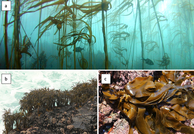
The PCFG display many foraging tactics and occupy several habitat types along the Oregon coast while they spend their summer feeding seasons here (Torres et al. 2018). Here, I will focus on one of these habitats: kelp. When you hear the word kelp, you probably conjure an image of long, thick stalks that reach from the ocean floor to the surface, with billowing fronds waving around (Figure 1a). However, this type is only one of three basic morphologies (Filbee-Dexter & Scheibling 2014) and it is called canopy kelp, which often forms extensive forests. The other two morphologies are stipitate and prostrate kelps. The former forms midwater stands (Figure 1b) while the latter forms low-lying kelp beds (Figure 1c). All three of these morphologies exist on the Oregon coast and create a mosaic of understory and canopy kelp patches that dot our coastline.
One of the most magnificent things about kelp is that it is not just a species itself, but it provides critical habitat, refuge, and food resources to a myriad of other species due to its high rates of primary production (Dayton 1985). Kelp is often referred to as a foundation species due to all of these critical services it provides. In Oregon, many species of rockfish, which are important commercial and recreational fisheries, use kelp as habitat throughout their life cycle, including as nursery grounds. Lingcod, another widely fished species, forages amongst kelp. A large number of macroinvertebrates can be found in Oregon kelp forests, including anemones, limpets, snails, sea urchins, sea stars, and abalone, to name a fraction of them.
Kelps grow best in cold, nutrient-rich waters (Tegner et al. 1996) and their growth and distribution patterns are highly naturally variable on both temporal and spatial scales (Krumhansl et al. 2016). However, warm water, low nutrient or light conditions, intensive grazing by herbivores, and severe storm activity can lead to the erosion and defoliation of kelp beds (Krumhansl et al. 2016). While these events can occur naturally in cyclical patterns, the frequency of several of these events has increased in recent years, as a result of climate change and anthropogenic impacts. For example, Dawn’s blog discussed increasing marine heatwaves that represent an influx of warm water for a prolonged period of time. In fact, kelps can be useful sentinels of change as they tend to be highly responsive to changes in environmental conditions (e.g., Rogers-Bennet & Catton 2019) and their nearshore, coastal location directly exposes them to human activities, such as pollution, harvesting, and fishing (Bennett et al. 2016).
Due to its foundational role, changes or impacts to kelp can reverberate throughout the ecosystem and negatively affect many other species. As mentioned previously, kelp is naturally highly variable, and like many other ecological processes, undergoes boom and bust cycles. For over four decades, dense, productive kelp forests have been shown to transition to sea urchin barrens, and back again, in natural cycles (Sala et al. 1998; Pinnegar et al. 2000; Steneck et al. 2002; Figure 2). These transitions are called phase shifts. In a healthy, balanced kelp forest, sea urchins typically passively feed on detrital plant matter, such as broken off pieces of kelp fronds that fall to the seafloor. A phase shift occurs when the grazing intensity of sea urchins increases, resulting in them actively feeding on kelp stalks and fronds to a point where the kelp in an area can become greatly reduced, creating an urchin barren. Sea urchin grazing intensity can change for a number of reasons, including reduction in sea urchin predators (e.g., sea otters, sunflower sea stars) or poor kelp recruitment events (e.g., due to warm water temperature). Regardless of the reason, the phases tend to transition back and forth over time. However, there is concern that sea urchin barrens may become an alternative stable state of the subtidal ecosystem from which kelp in an area cannot recover (Filbee-Dexter & Scheibling 2014).

For example, in 2014, bull kelp canopy cover in northern California was reduced by >90% and has not shown signs of recovery since (Rogers-Bennet & Catton 2019; Figure 3). This massive decline was attributed to two major events: 1) the onset of sea star wasting disease (SSWD) in 2013 and 2) the “warm blob” of 2014-2016. SSWD affected over 20 sea star species along the coast from Mexico to Alaska, with the predatory sunflower sea star, which consumes purple sea urchins, most affected, including population declines of 80-100% along the coast (Harvell et al. 2019). Following this SSWD outbreak, the “warm blob”, which was an extreme marine heatwave in the Pacific Ocean, caused ocean temperatures to spike. These two events allowed purple sea urchin populations to grow unchecked by their predators, and created nutrient-poor and warm water conditions, which limited kelp growth and productivity. Intense grazing on bull kelp by growing urchin populations resulted in the >90% reduction in bull kelp canopy cover and has left behind widespread urchin barrens instead (Rogers-Bennet & Catton 2019). Consequently, there have been ecological and economic impacts on the ecosystem and communities in northern California. Without bull kelp, red abalone and red sea urchin populations starved, leading to a subsequent loss of the recreational red abalone (estimated value of $44 million/year) and commercial red urchin fisheries in northern California (Rogers-Bennet & Catton 2019).

As I mentioned earlier, while phase shifts between kelp forests and urchin barrens are common cycles, the intensity of the events described above in northern California are an example of sea urchin barrens potentially becoming a stable state of the subtidal ecosystem (Filbee-Dexter & Scheibling 2014). Given that marine heatwaves are only expected to increase in intensity and frequency in the future (Frölicher et al. 2018), the events documented in northern California may not be an isolated incidence.
Considering that parts of the Oregon coast, particularly the southern portion, are very similar to northern California biogeographically, and that it was not exempt from the “warm blob”, similar changes in kelp forests may be occurring along our coast. There are many individuals and groups that are actively working on this issue to examine potential impacts to kelp and the species that depend on the services it provides. For more information, check out the Oregon Kelp Alliance.

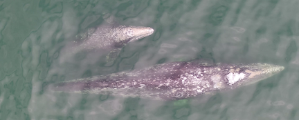
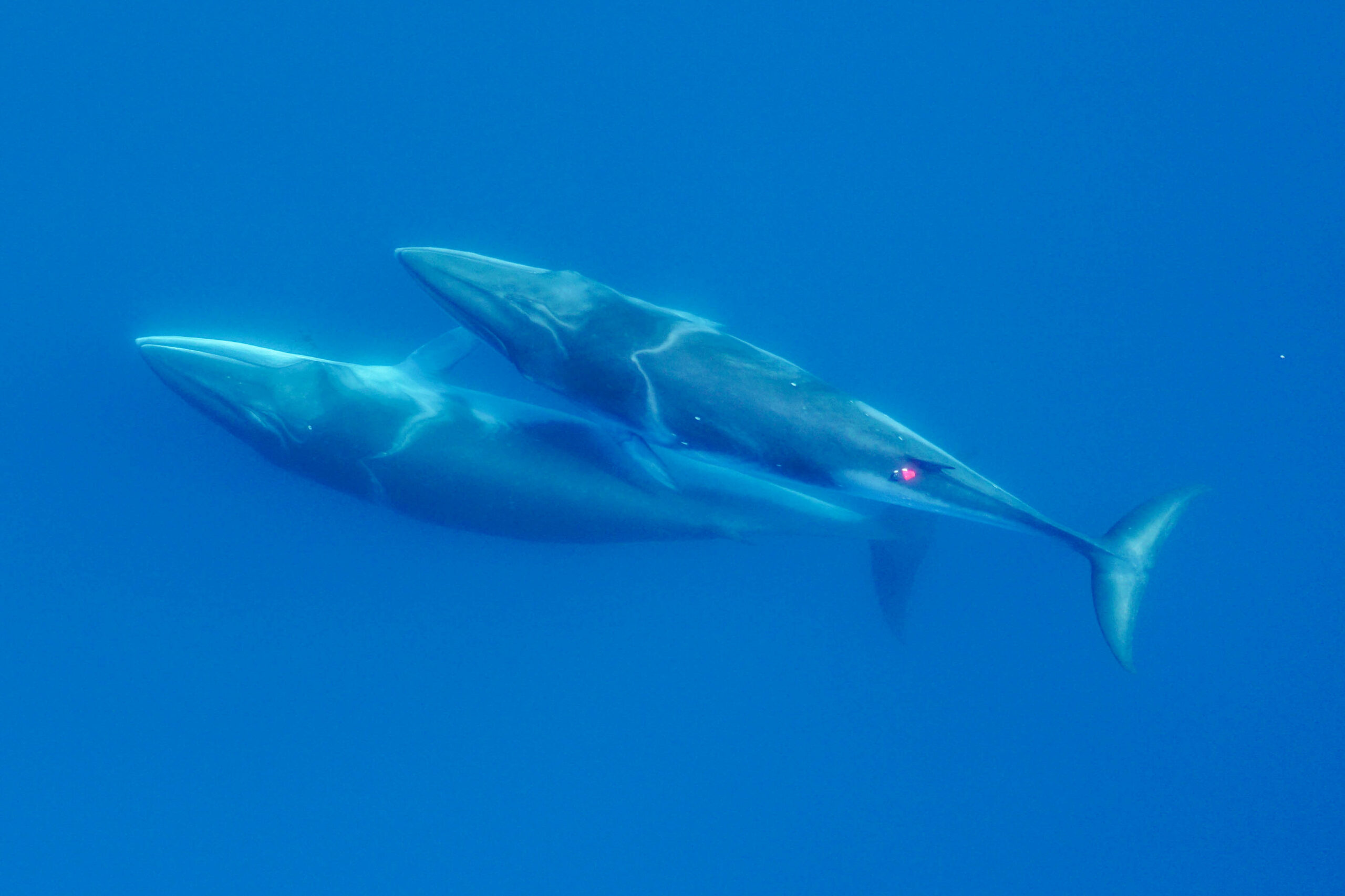
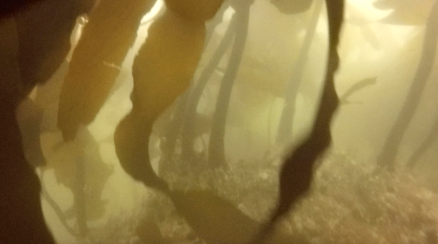
So, what does all of this information have to do with gray whales? Given their affinity for kelp habitats (Figure 4) and their zooplankton prey that aggregates there, changes to kelp ecosystems may affect gray whale health and ecology. This aspect of the complex kelp trophic web has not been examined to date; thus one of my PhD chapters focuses on the response of gray whales to changing kelp ecosystems along the southern Oregon coast. To do this, I am examining 6 years of data collected during the TOPAZ/JASPER project in Port Orford, to look at the relationships between kelp health, sea urchin density, zooplankton abundance, and gray whale foraging effort over space and time. Documenting impacts of changing kelp forests on gray whales is important to assist management efforts as healthy and abundant kelp seems critical in providing ample food opportunities for these iconic Pacific Northwest marine predators.
Did you enjoy this blog? Want to learn more about marine life, research, and conservation? Subscribe to our blog and get a weekly alert when we make a new post! Just add your name into the subscribe box on the left panel.
References
Bennett S, et al. The ‘Great Southern Reef’: Social, ecological and economic value of Australia’s neglected kelp forests. Marine and Freshwater Research 67:47-56.
Dayton PK (1985) Ecology of kelp communities. Annual Review of Ecology and Systematics 16:215-245.
Filbee-Dexter K, Scheibling RE (2014) Sea uechin barrens as alternative stable states of collapsed kelp ecosystems. Marine Ecology Progress Series 495:1-25.
Frölicher TL, Fischer EM, Gruber N (2018) Marine heatwaves under global warming. Nature 560:360-364.
Harvell CD, et al. (2019) Disease epidemic and a marine heat wave are associated with the continental-scale collapse of a pivotal predator (Pycnopodia helianthoides). Science Advances 5(1) doi:10.1126/sciadv.aau7042.
Krumhansl KA, et al. (2016) Global patterns of kelp forest change over the past half-century. Proceedings of the National Academy of Sciences of the United States of America 113(48):13785-13790.
Pinnegar JK, et al. (2000) Trophic cascades in benthic marine ecosystems: lessons for fisheries and protected-area management. Environmental Conservation 27:179-200.
Rogers-Bennett L, Catton CA (2019) Marine heat wave and multiple stressors tip bull kelp forest to sea urchin barrens. Scientific Reports 9:15050.
Sala E, Boudouresque CF, Harmelin-Vivien M (1998) Fishing, trophic cascades and the structure of algal assemblages; evaluation of an old but untested paradigm. Oikos 82:425-439.
Steneck RS, et al. (2002) Kelp forest ecosystems: biodiversity, stability, resilience and future. Environmental Conservation 29:436-459.
Tegner MJ, Dayton PK, Edwards PB, Riser KL (1996) Is there evidence for the long-term climatic change in southern California kelp forests? California Cooperative Oceanic Fisheries Investigations Report 37:111-126.
Torres LG, Nieukirk SL, Lemos L, Chandler TE (2018) Drone up! Quantifying whale behavior from a new perspective improves observational capacity. Frontiers in Marine Science doi:10.3389/fmars.2019.00319.