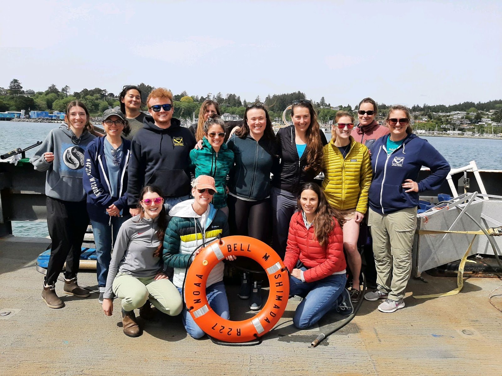
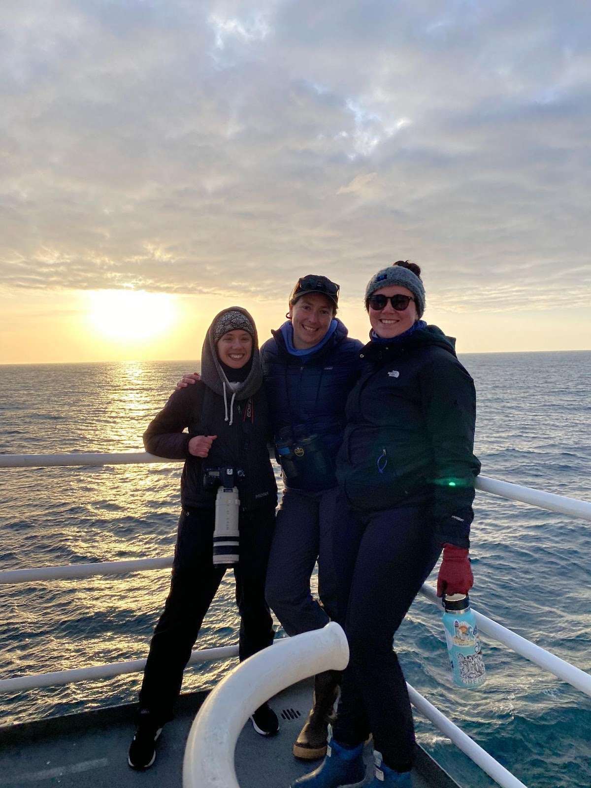
By Dawn Barlow, Postdoctoral Scholar, OSU Department of Fisheries, Wildlife, and Conservation Sciences, Geospatial Ecology of Marine Megafauna Lab
Global climate change is affecting all aspects of life on earth. The oceans are not exempt from these impacts. On the contrary, marine species and ecosystems are experiencing significant impacts of climate change at faster rates and greater magnitudes than on land1,2, with cascading effects across trophic levels, impacting human communities that depend on healthy ocean ecosystems3.
In the lobby of the Gladys Valley Marine Studies building that we are privileged to work in here at the Hatfield Marine Science Center, a poem hangs on the wall: “The North Pacific Is Misbehaving”, by Duncan Berry. I read it often, each time moved by how he articulates both the scientific curiosity and the personal emotion that are intertwined in researchers whose work is dedicated to understanding the oceans on a rapidly changing planet. We seek to uncover truths about the watery places we love that capture our fascination; truths that are sometimes beautiful, sometimes puzzling, sometimes heartbreaking. Observations conducted with scientific rigor do not preclude complex human feelings of helplessness, determination, and hope.

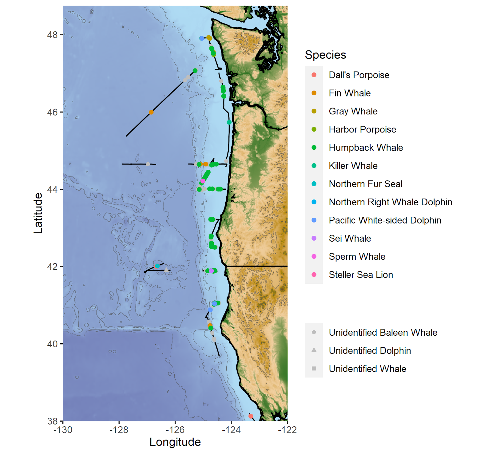
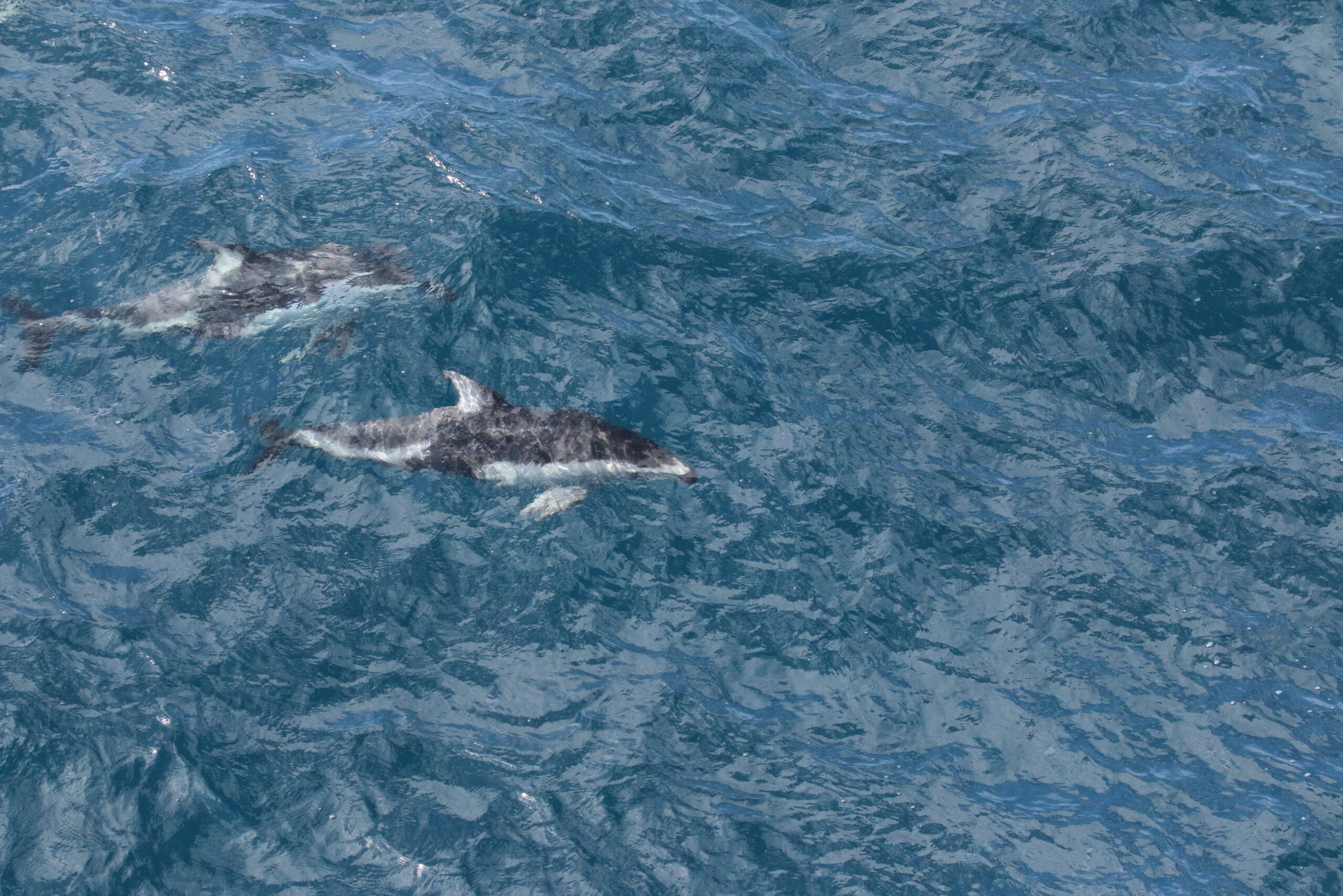
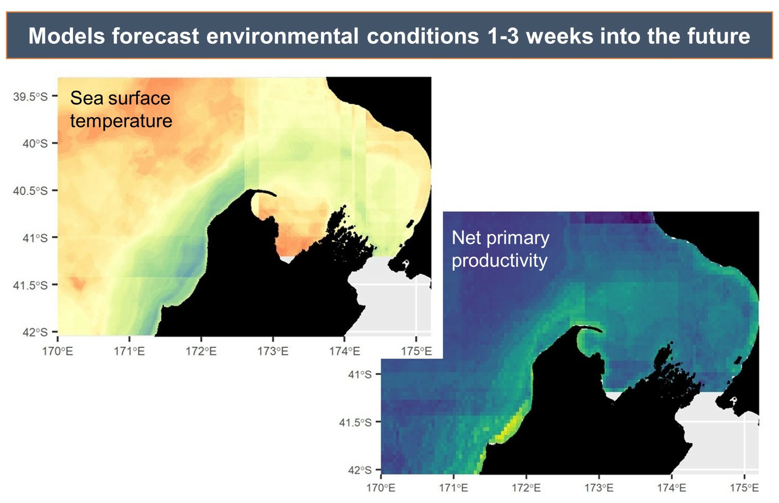
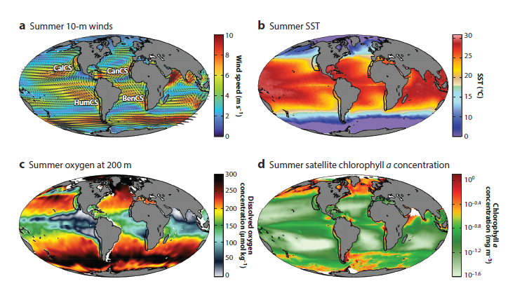
Here on the Oregon Coast, we are perched on the edge of a bountiful upwelling ecosystem. Upwelling is the process by which winds drive a net movement of surface water offshore, which is replaced by cold, nutrient-rich water. When this water full of nutrients meets the sunlight of the photic zone, large phytoplankton blooms occur that sustain high densities of forage species like zooplankton and fish, and yielding important feeding opportunities for predators such as marine mammals. Upwelling ecosystems, like the California Current system in our back yard that features in Duncan Berry’s poem, support over 20% of global fisheries catches despite covering an area less than 5% of the global oceans4–6. These narrow bands of ocean on the eastern boundaries of the major oceans are characterized by strong winds, cool sea surface temperatures, and high primary productivity that ultimately support thriving and productive ecosystems (Fig. 2)7.
Because of their importance to human societies, eastern boundary current upwelling systems (EBUSs) have been well-studied over time. Now, scientists around the world who have dedicated their careers to understanding and describing the dynamics of upwelling systems are forced to reckon with the looming question of what will happen to these systems under climate change. The state of available information was recently synthesized in a forthcoming paper by Bograd et al. (2023). These authors find that the future of upwelling systems is uncertain, as climate change is anticipated to drive conflicting physical changes in their oceanography. Namely, alongshore winds could increase, which would yield increased upwelling. However, a poleward shift in these upwelling systems will likely lead to long-term changes in the intensity, location, and seasonality of upwelling-favorable winds, with intensification in poleward regions but weakening in equatorward areas. Another projected change is stronger temperature gradients between inshore and offshore areas, and vertically within the water column. What these various opposing forces will mean for primary productivity and species community structure remains to be seen.
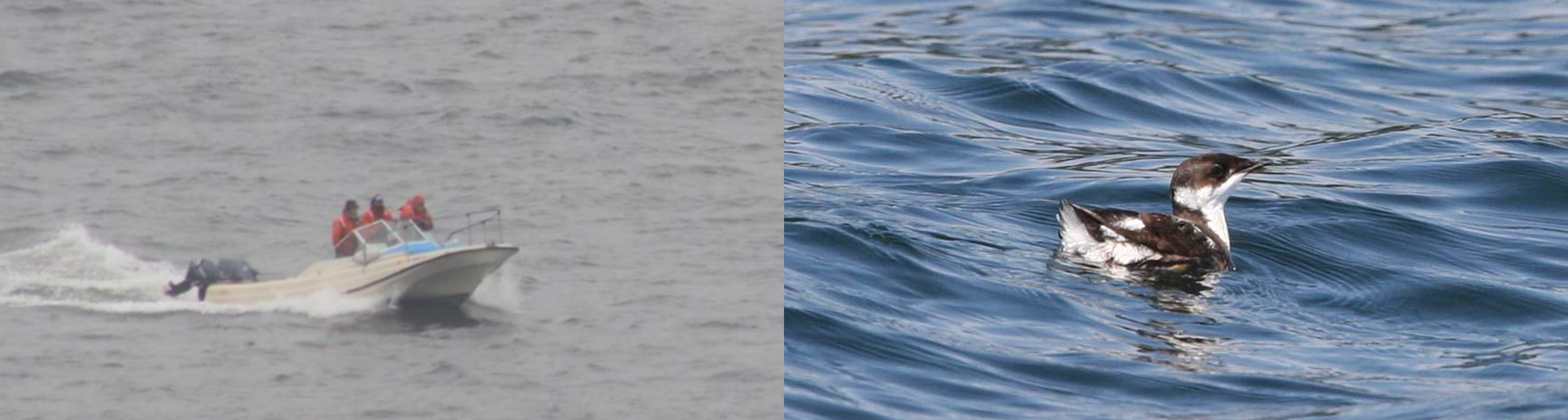
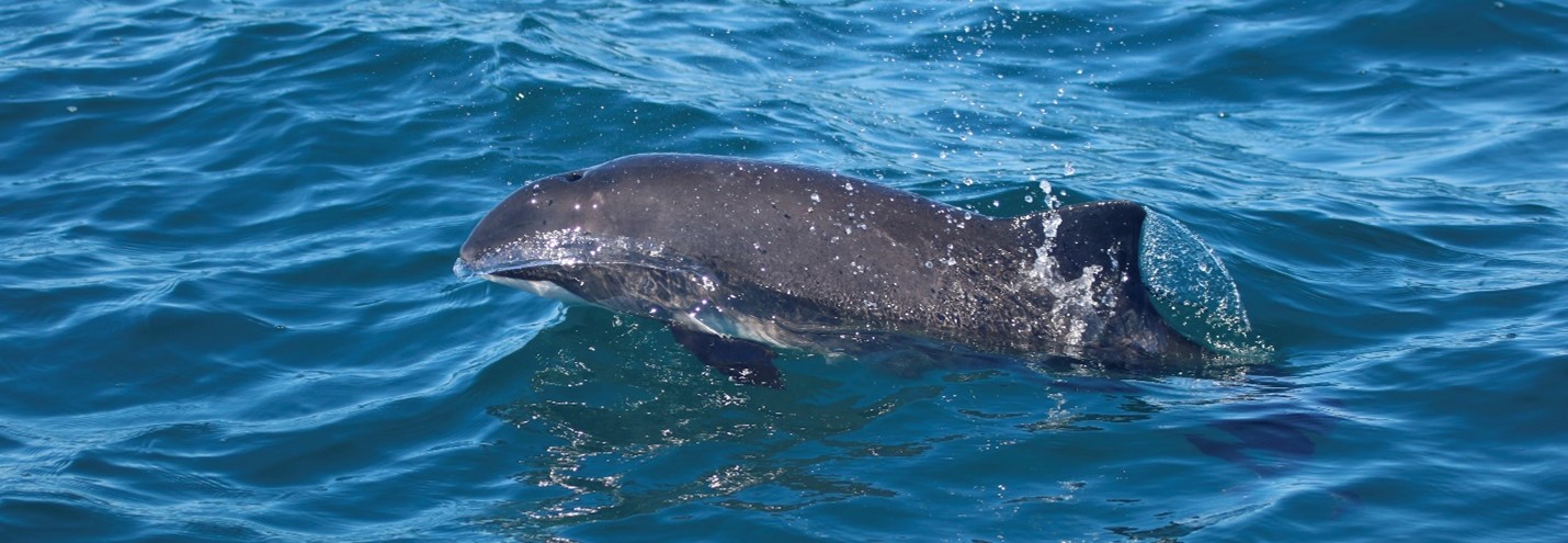
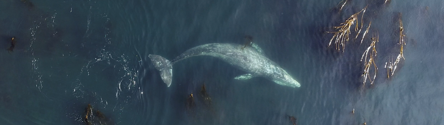
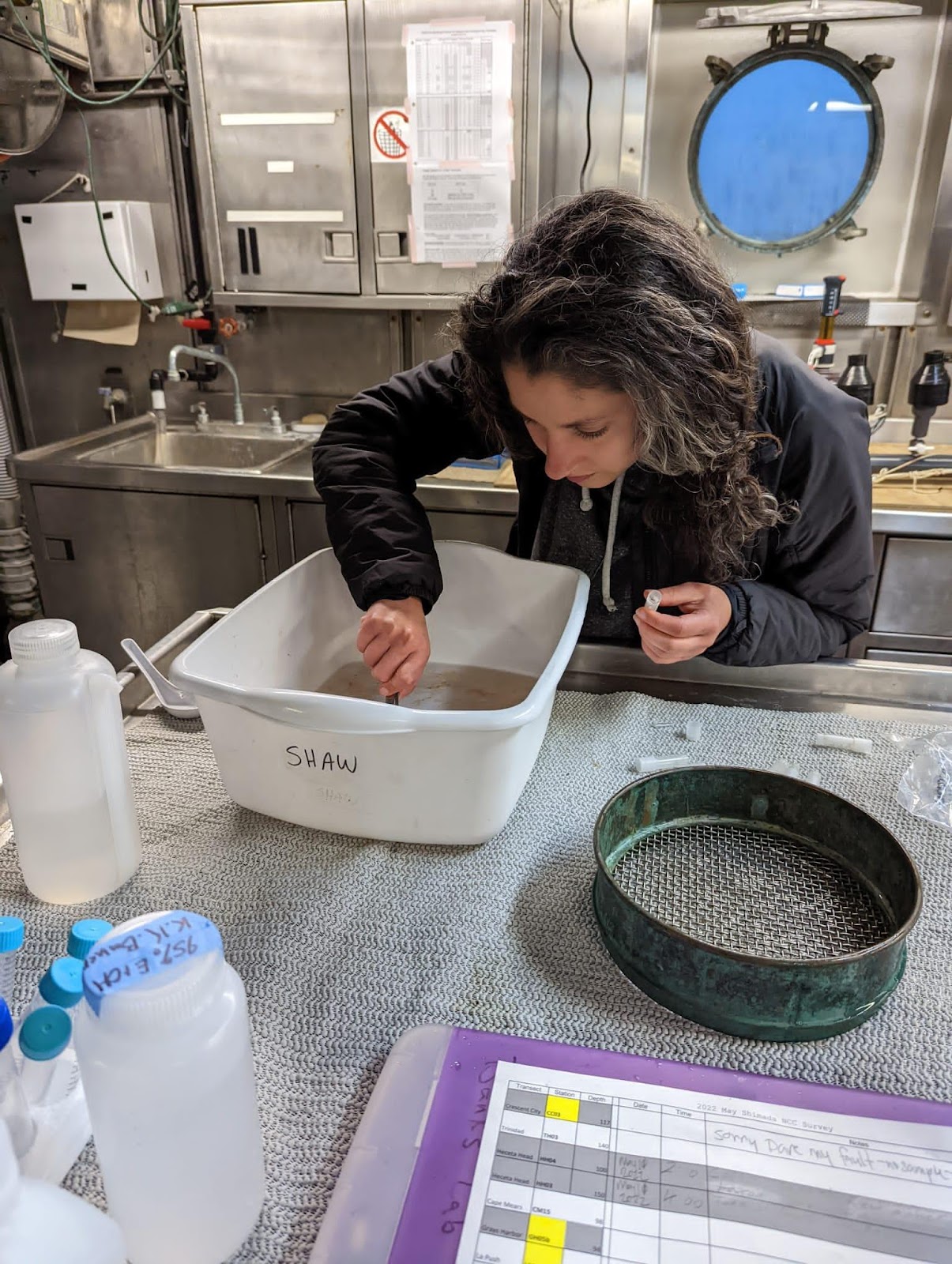
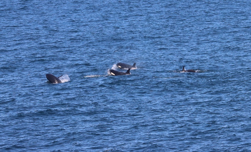
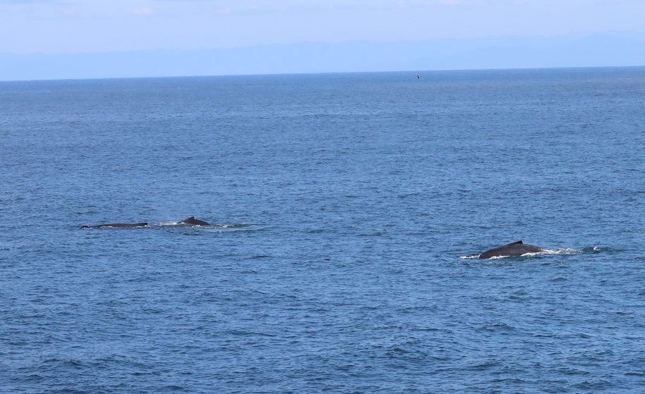
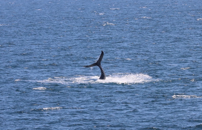
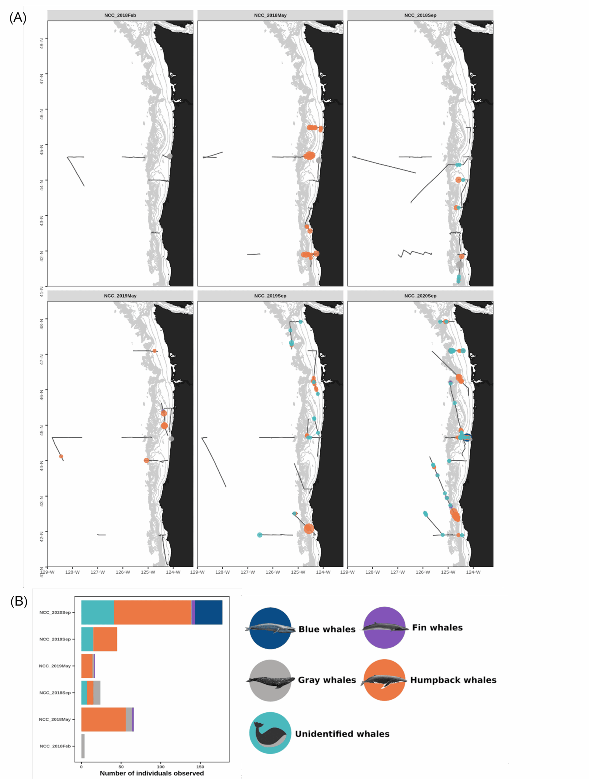
While most of my prior research has centered around the importance of productive upwelling systems for supporting marine mammal feeding grounds8–10, my recent focus has shifted closer to home, to the nearshore waters less than 5 km from the coastline. Despite their ecological and economic importance, nearshore habitats remain understudied, particularly in the context of climate change. Through the recently launched EMERALD project, we are investigating spatial and temporal distribution patterns of harbor porpoises and gray whales between San Francisco Bay and the Columbia River in relation to fluctuations in key environmental drivers over the past 30 years. On a scientific level, I am thrilled to have such a rich dataset that enables asking broad questions relating to how changing environmental conditions have impacted these nearshore sentinel species. On a more personal level, I must admit some apprehension of what we will find. The excitement of detecting statistically significant northward shift in harbor porpoise distribution stands at odds with my own grappling with what that means for our planet. The oceans are changing, and sensitive species must move or adapt to persist. What does the future hold for this “wild edge of a continent of ours” that I love, as Duncan Berry describes?
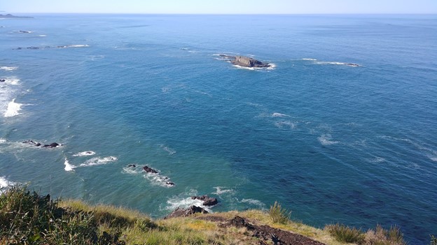
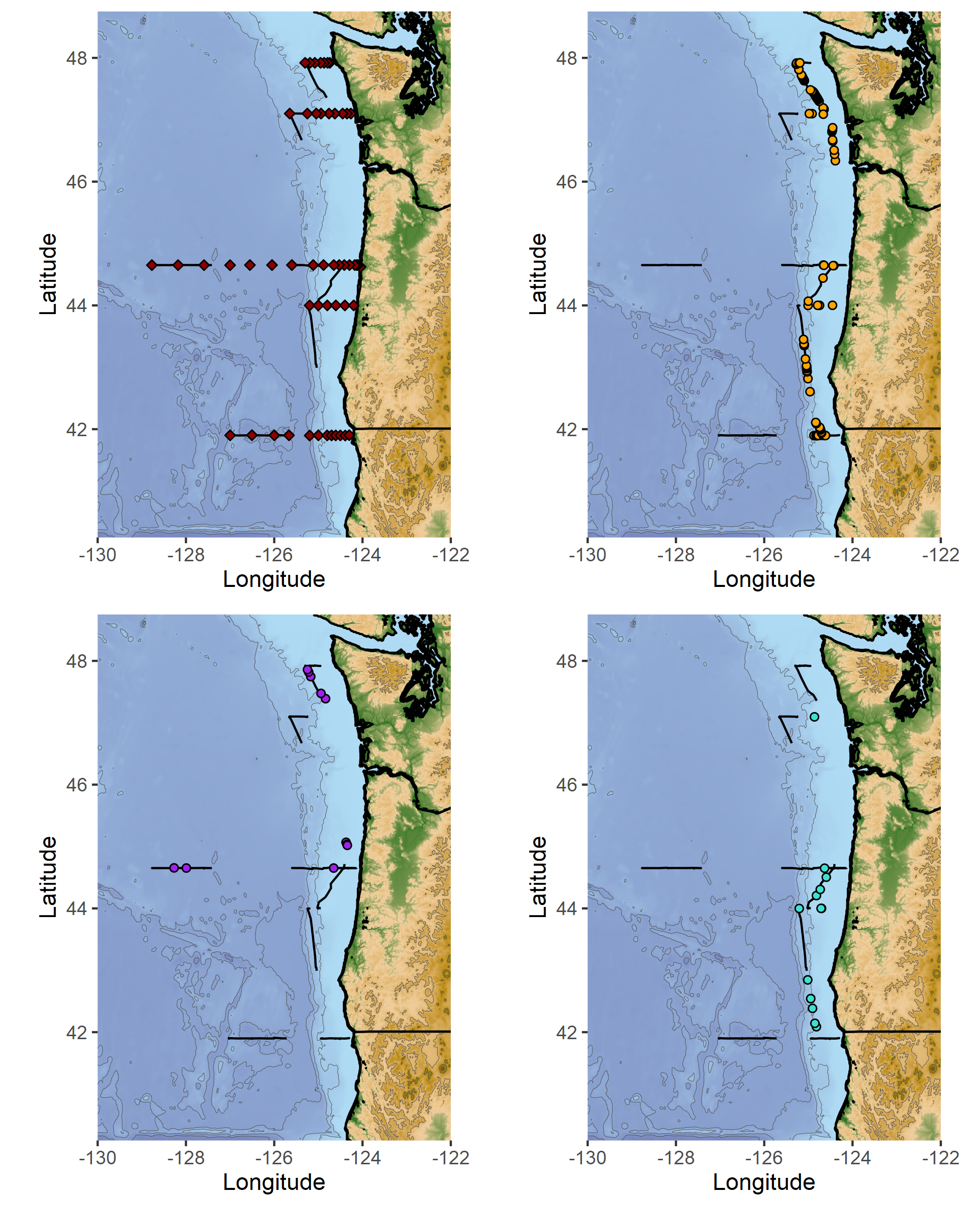
Evidence exists that the nearshore realm of the Northeast Pacific is actually decoupled from coastal upwelling processes11. Rather, these areas may be a “sweet spot” in the coastal boundary layer where headlands and rocky reefs provide more stable retention areas of productivity, distinct from the strong upwelling currents just slightly further from shore (Fig. 4). As the oceans continue to shift under the impacts of climate change, what will it mean for these critically important nearshore habitats? While they are adjacent to prominent upwelling systems, they are also physically, biologically, and ecologically distinct. Will nearshore habitats act as a refuge alongside a more rapidly changing upwelling environment, or will they be impacted in some different way? Many unanswered questions remain. I am eager to continue seeking out truth in the data, with my drive for scientific inquiry fueled by my underlying connection to this wild edge of a continent that I call home.
Did you enjoy this blog? Want to learn more about marine life, research, and conservation? Subscribe to our blog and get a weekly alert when we make a new post! Just add your name into the subscribe box below!
References:
1. Poloczanska, E. S. et al. Global imprint of climate change on marine life. Nat. Clim. Chang. 3, (2013).
2. Lenoir, J. et al. Species better track climate warming in the oceans than on land. Nat. Ecol. Evol. 4, 1044–1059 (2020).
3. Hoegh-Guldberg, O. & Bruno, J. F. The impact of climate change on the world’s marine ecosystems. Science (2010). doi:10.1126/science.1189930
4. Mann, K. H. & Lazier, J. R. N. Dynamics of Marine Ecosystems: Biological-physical interactions in the oceans. Blackwell Scientific Publications (1996). doi:10.2307/2960585
5. Ryther, J. Photosynthesis and fish production in the sea. Science (80-. ). 166, 72–76 (1969).
6. Cushing, D. H. Plankton production and year-class strength in fish populations: An update of the match/mismatch hypothesis. Adv. Mar. Biol. 9, 255–334 (1990).
7. Bograd, S. J. et al. Climate Change Impacts on Eastern Boundary Upwelling Systems. Ann. Rev. Mar. Sci. 15, 1–26 (2023).
8. Barlow, D. R., Bernard, K. S., Escobar-Flores, P., Palacios, D. M. & Torres, L. G. Links in the trophic chain: Modeling functional relationships between in situ oceanography, krill, and blue whale distribution under different oceanographic regimes. Mar. Ecol. Prog. Ser. 642, 207–225 (2020).
9. Barlow, D. R., Klinck, H., Ponirakis, D., Garvey, C. & Torres, L. G. Temporal and spatial lags between wind, coastal upwelling, and blue whale occurrence. Sci. Rep. 11, 1–10 (2021).
10. Derville, S., Barlow, D. R., Hayslip, C. & Torres, L. G. Seasonal, Annual, and Decadal Distribution of Three Rorqual Whale Species Relative to Dynamic Ocean Conditions Off Oregon, USA. Front. Mar. Sci. 9, 1–19 (2022).
11. Shanks, A. L. & Shearman, R. K. Paradigm lost? Cross-shelf distributions of intertidal invertebrate larvae are unaffected by upwelling or downwelling. Mar. Ecol. Prog. Ser. 385, 189–204 (2009).