A Journey From Microbiology to Macrobiology

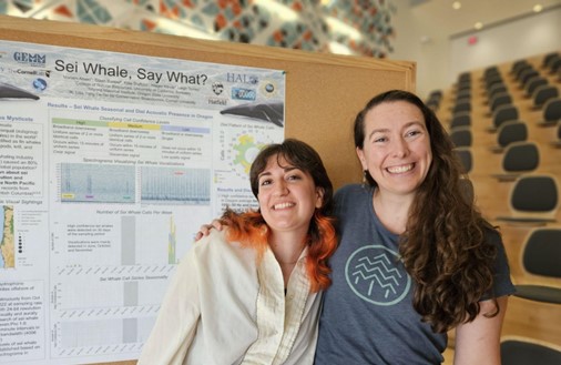
Mariam Alsaid, University of California Berkeley, GEMM Lab REU Intern

My name is Mariam Alsaid and I am currently a 5th year undergraduate transfer student at the University of California, Berkeley. Growing up on the small island of Bahrain, I was always minutes away from the water and was enraptured by the creatures that lie beneath the surface. Despite my long-standing interest in marine science, I never had the opportunity to explore it until just a few months ago. My professional background up until this point was predominantly in soil microbiology through my work with Lawrence Berkeley National Laboratory, and I was anxious about how I would switch directions and finally be able to pursue my main passion. For this reason, I was thrilled by my acceptance into the OSU Hatfield Marine Science Center’s REU program this year, which led to my exciting collaboration with the GEMM Lab. It was kind of a silly transition to go from studying bacteria, one of the smallest organisms on earth, to whales, who are the largest.

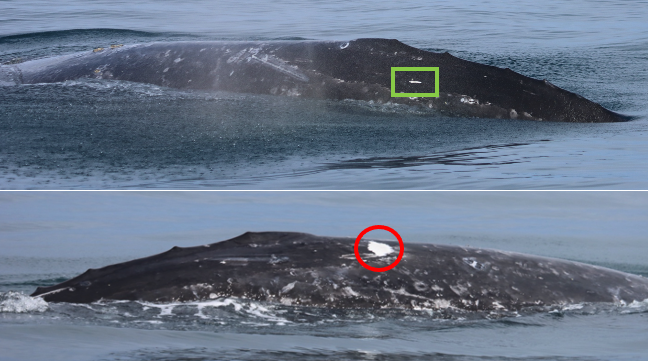
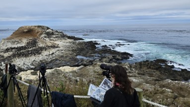
My project this summer focused on sei whale acoustic occurrence off the coast of Oregon. “What’s a sei whale?” is a question I heard a lot throughout the summer and is one that I had to Google myself several times before starting my internship. Believe it or not, sei whales are the third largest rorqual in the world but don’t get much publicity because of their small population sizes and secretive behavior. The commercial whaling industry of the 19th and 20th centuries did a number on sei whale populations globally, rendering them endangered. In consequence, little research has been conducted on their global range, habitat use, and behavior since the ban of commercial whaling in 1986 (Nieukirk et al. 2020). Additionally, sei whales are relatively challenging to study because of their physical similarities to the fin whale, and acoustic similarities to other rorqual vocalizations, most notably blue whale D-calls and fin whale 40 Hz calls. As of today, published literature indicates that sei whale acoustic presence in the Pacific Ocean is restricted to Antarctica, Chile, Hawaii, and possibly British Columbia, Canada (Mcdonald et al. 2005; Espanol-Jiminez et al. 2019; Rankin and Barlow, 2012; Burnham et al. 2019). The idea behind this research project was sparked by sparse visual sightings of sei whales by research cruises conducted by the Marine Mammal Institute (MMI) in recent years (Figure 1). This raised questions about if sei whales are really present in Oregon waters (and not just misidentified fin whales) and if so, how often?

*Figure 1. Map of sei whale visual sightings off the coast of Oregon, colored by MMI Lab research cruise, and the location of the hydrophone at NH45 (white star).*

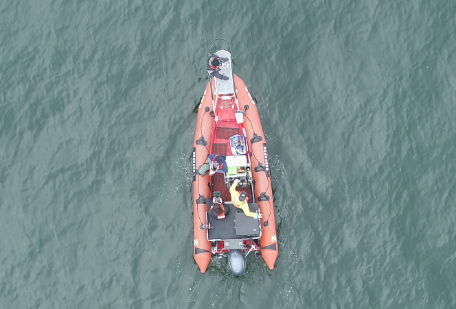
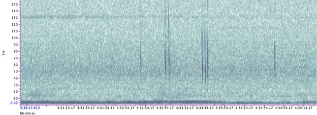
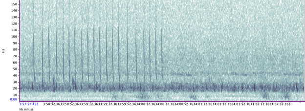
A hydrophone, which is a fancy piece of equipment that records continuous underwater sound, was deployed 45 miles offshore of Newport, OR between October of 2021 and December of 2022. My role this summer was to use this acoustic data to determine whether sei whales are hanging out in Oregon or not. Acoustic data was analyzed using the software Raven Pro, which allowed me to visualize sound in the form of spectrograms (Fig. 2). From there, my task was to select signals that could potentially be sei whale calls. It was a hurdle familiarizing myself with sei whale vocalizations while also keeping in mind that other species (e.g., blue and fin whales) may produce similar sounding (and looking in the spectrograms) calls. For this reason, I decided to establish confidence levels based on published sei whale acoustic research that would help me classify calls with less bias. Vocalizations produced by sei whales are characterized by low frequency, broadband, downsweeps. Sei whales can be acoustically distinguished from other whales because of their tendency to produce uniform groups of calls (typically in doublets and triplets) in a short timeframe. This key finding allowed me to navigate the acoustic data with more ease.

The majority of the summer was spent slowly scanning through the months of data at 5-minute increments. As you can imagine, excitement varied by day. Some days I would find insanely clear signals of blue, fin, and humpback whales and other days I would find nothing. The major discovery and the light at the end of the tunnel was the SEI WHALES!!! I detected numerous high quality sei whale calls throughout the study period with peaks in October and November (but a significantly higher peak in occurrence in 2022 versus 2021). I also encountered a unique vocalization type in fall of 2022, consisting of a very long series of repeated calls that we called “multiplet”, rather than doublets or triplets that is more typical of sei whales (Fig. 3). Lastly, I found no significant diel pattern in sei whale vocalization, indicating that these animals call at any hour of the day. More research needs to go into this project to better estimate sei whale occurrence and understand their behavior in Oregon but this preliminary work provides a great baseline into what sei whales sound like in this part of the world. In the future, the GEMM lab intends on implementing more hydrophone data and work on developing an automated detection system that would identify sei whale calls automatically.

*Figure 2. Spectrogram of typical sei whale calls detected in acoustic data*

*Figure 3. Spectrogram of unique sei whale multiplet call type*

*Figure 4. My first time conducting fieldwork! I spent a few mornings assisting Dr. Rachel Orben’s group in surveying murre and cormorant nests (thanks to my good friend Jacque McKay :))*

My experience this summer was so formative for me. As someone who has been an aspiring marine biologist for so long, I am so grateful for my experience working with the GEMM Lab alongside incredible scientists who are equally passionate about studying the mysteries of the ocean. This experience has also piqued my interest in bioacoustics and I plan on searching for other opportunities to explore the field in the future. Aside from growing professionally, I learned that I am more capable of tackling and overcoming obstacles than I had thought. I was afraid of entering a field that I knew so little about and was worried about failing and not fitting in. My anxieties were overshadowed by the welcoming atmosphere at Hatfield and I could not have asked for better people to work with. As I was searching for sei whale calls this summer, I suppose that I was also unintentionally searching for my voice as a young scientist in a great, blue field.

*Figure 5. My mentor, Dr. Dawn Barlow, and I with my research poster at the Hatfield Marine Science Center Coastal Intern Symposium*

Did you enjoy this blog? Want to learn more about marine life, research, and conservation? Subscribe to our blog and get a weekly alert when we make a new post! Just add your name into the subscribe box below!

References:

Nieukirk, S. L., Mellinger, D. K., Dziak, R. P., Matsumoto, H., & Klinck, H. (2020). Multi-year occurrence of sei whale calls in North Atlantic polar waters. The Journal of the Acoustical Society of America, 147(3), 1842–1850. https://doi.org/10.1121/10.0000931

McDonald, M. A., Calambokidis, J., Teranishi, A. M., & Hildebrand, J. A. (2001). The acoustic calls of blue whales off California with gender data. The Journal of the Acoustical Society of America, 109(4), 1728–1735. https://doi.org/10.1121/1.1353593

Español-Jiménez, S., Bahamonde, P. A., Chiang, G., & Häussermann, V. (2019). Discovering sounds in Patagonia: Characterizing sei whale (<i>Balaenoptera borealis</i>) downsweeps in the south-eastern Pacific Ocean. Ocean Science, 15(1), 75–82. https://doi.org/10.5194/os-15-75-2019

Rankin, S., & Barlow, J. (2007). VOCALIZATIONS OF THE SEI WHALE BALAENOPTERA BOREALIS OFF THE HAWAIIAN ISLANDS. Bioacoustics, 16(2), 137–145. https://doi.org/10.1080/09524622.2007.9753572

Burnham, R. E., Duffus, D. A., & Mouy, X. (2019). The presence of large whale species in Clayoquot Sound and its offshore waters. Continental Shelf Research, 177, 15–23. https://doi.org/10.1016/j.csr.2019.03.004

Exploring the Western Antarctic Peninsula

By Abby Tomita, undergraduate student, OSU College of Earth, Ocean, and Atmospheric Sciences, research intern in the GEMM and Krill Seeker Labs

This February, during the winter term of my third year at Oregon State, I was presented with a once-in-a-lifetime opportunity. After spending the last year studying the zooplankton krill as part of Project OPAL, I was invited to spend the austral winter season doing research on Antarctic krill (Euphausia superba) under supervision of experts Dr. Kim Bernard and PhD student Rachel Kaplan. Additionally, we were lucky enough to participate in two research cruises along the Western Antarctic Peninsula (WAP).

Figure 1. Sailing into the sunset on the RV *Laurence M. Gould*.

Unsurprisingly, it is no easy feat getting to the bottom of the world. After an incredibly thorough physical qualification process and two days of air travel from Portland, Oregon, we reached the lovely city of Punta Arenas, Chile. It was such a relief to arrive – but we were only halfway there. The next portion of our trip was the one that I was most anxious about, especially as someone who is prone to seasickness: crossing the Drake Passage. This stretch of the ocean, from the southernmost tip of South America to the Antarctic Peninsula, is notoriously treacherous as water in this area circulates the globe completely unobstructed by land masses. I soon learned the value of scopolamine patches and nausea bracelets, which helped me immensely through this five day journey. From Punta Arenas, we boarded the RV Laurence M. Gould, along with a seal research team from the University of North Carolina Wilmington. They were headed down south to look for crabeater seals to better understand not only their physiology, but also their role in the trophic ecology of the WAP.

The Passage was rough, but not as terrible as I expected. The hype around it made me think I’d be faced with something as menacing as the giant wave from The Perfect Storm, and while the rocking and rolling of the ship was far from pleasant, my nausea aids, as well as the amazing people and vast selection of movies on board made it manageable. Despite being extremely nervous for the Passage, I was also very excited to celebrate my twenty-first birthday during it. It was a memorable, although untraditional birthday experience that was made all the more special by my friends on the ship who took the time to celebrate the day as best as we could.

Figure 2. Taking in the sights of the Neumayer Channel with Kim!

The morning that we reached the Bransfield Strait was something truly unforgettable. Up until that point, I knew our destination was Antarctica, but I couldn’t really wrap my head around it because it was such a distant place and concept to me. I remember walking out onto the starboard side of the second level deck and seeing huge mountains out in the distance. For some reason, I had never considered how massively tall the mountains of the peninsula are, and just the fact that there were mountains down here at all. I joined the others at the bow, where we stood for hours in awe at the first land we had seen in days. Though many of the other scientists and crew members on board had been to this icy continent before, this was my first time, and I was in a state of disbelief. We’d finally made it and it sunk into me that I was in Antarctica, and that I would be here for the next five and half months.

After a day of hiding from strong winds in the Neumayer Channel, we were able to dock at Palmer Station (the smallest of the three US research bases in Antarctica) for our first port call, and seeing Palmer for the first time was just as exciting as seeing the continent. It looked so small at first, especially with the glacier and mountains looming behind it. Once the ship was tied up, orientation began. The station manager came onto the ship to give us an overview of what we could expect on station and the general Palmer etiquette. Next, we were given a tour of the facilities, from the lab spaces and aquarium room, up through the galley/dining area, past the hot tub and sauna, and into the lounge and bar in the GWR (Garage, Warehouse, and Recreation) building. I was surprised at how cozy the station was on the inside. In pictures, the buildings’ exteriors looked similar to the outside of a metal shipping container, but the inside was welcoming and warm. Those of us staying on station then sat through several hours of a more detailed orientation that somehow wore us out despite sitting in comfy recliner sofas the whole time. After sleeping on the rocking ship for about a week, I had some of the best sleep of my life that first night at Palmer Station.

Figure 3. Arriving at the Palmer Station pier in the first morning light.

Our first research cruise started a few days after arriving at Palmer, and just like that, we were off to explore the Southern Ocean. This leg of the trip took us south, down to Marguerite Bay and the region of Alexander Island, for ten days. The views were just spectacular everywhere we went, and it was so humbling to step out onto the deck to see gigantic mountains all around the ship. By day, us “krillers”, as our team is known, camped out on the bridge of the ship with the seal team, where we looked for sea ice floes with lounging crabeater seals. By night we conducted CTD casts, filtered water for chlorophyll, and deployed nets to catch our favorite tiny crustacean critters, along with any other zooplankton in our track. Unfortunately for both our group and the seal team, many areas that we visited were not frequented by krill or crabeater seals, though the seal team did successfully study and tag one seal over the course of the first cruise.

Figure 4. Rachel (right) and I (left) filtering water for chlorophyll on the LMG.

One of the highlights of this leg of the cruise was our Crossing Ceremony, as we’d crossed the Antarctic Circle (approximately 66.5ºS) shortly after leaving Palmer station. Myself and six others were crossing for the first time, so to earn our “Red Noses”, we had to pay tribute to King Neptune and his court. It would not be a Crossing Ceremony without at least some light pranking, so when they brought us out individually to the main deck, I knew something was coming our way.

Figure 5. Taking a celebratory picture with King Neptune’s court…with a surprise after.

The ten days flew by, and when we arrived back on station, we had less than a week to prepare for our next excursion on the LMG, which would be fifteen days. The time back at Palmer went quickly as we organized our lab space and entered data from the first cruise. The ship came back once more and we were off, this time heading north along the Peninsula to the Gerlache Strait. The sights were as breathtaking as ever, and I was excited to be back with my friends from the ship.

Figure 6. Kim (left) and I (right) pour krill we caught into an XACTIC tank.

Our first day of transit was through the Lemaire Channel, one of the most stunning areas that we passed through (check out the photo gallery at the end of this post!). We spent the majority of the day on the bow and the deck of the bridge taking in the beautiful towering mountains on either side of the narrow channel and watching for penguins and humpbacks, of which there were many. This voyage segued into an extremely productive night of science for us where we caught thousands of krill that we were able to keep live in tanks on the ship, in preparation for later use for our experiments on station. Our first productive night of science was auspicious for the rest of the cruise as we caught and processed thousands more krill, and the seal team had a much more fruitful experience finding crabeater seals (they found/worked on 8 seals and named them all after fruits!). The highlight of this second cruise for me was getting to accompany the seal team onto an ice floe in the Lemaire Channel to assist them in their work on the crabeater, a female juvenile who they named Mango!

Figure 7. Watching Mango’s nose to calculate and record her breaths per minute (US NMSF Permit #25770).

Returning to Palmer for the final time on the LMG was just as exciting as arriving the first time, especially with the knowledge that we’d have one last night of celebration with our friends from the ship at the Cross Town Dinner – a night to celebrate the solstice with both the Palmer crew and LMG crew. Although the dinner and subsequent party were a blast, I felt a lingering sadness knowing that the majority of the people I spent almost two months with would be heading north, back to their respective homes while Kim, Rachel, and I stayed at Palmer for the next few months. The next day, after saying our goodbyes, the three of us stood on the Palmer pier with tears streaming down our faces, waving frantically at the ship to our friends on the deck. In spite of my sadness, I knew that the coming months would be a thrilling series of new experiences in one of the most magical and special places that I have ever had the pleasure of being in.

Figure 8. The LMG departs Palmer Station for the last time this winter!

Familiar flukes and flanks: The 9th GRANITE field season is underway

By Lisa Hildebrand, PhD student, OSU Department of Fisheries, Wildlife, & Conservation Sciences, Geospatial Ecology of Marine Megafauna Lab

The winds are consistently (and sometimes aggressively) blowing from the north here on the Oregon coast, which can only mean one thing – summer has arrived! Since mid-May, the GRANITE (Gray whale Response to Ambient Noise Informed by Technology and Ecology) team has been looking for good weather windows to survey for gray whales and we have managed to get five great field work days already. In today’s blog post, I am going to share what (and who) we have seen so far.

On our first day of the field season, PI Leigh Torres, postdoc KC Bierlich and myself, were joined by a special guest: Dr. Andy Read. Andy is the director of the Duke University Marine Lab, where he also runs his own lab, which focuses on conservation biology and ecology of marine vertebrates. Andy was visiting the Hatfield Marine Science Center as part of the Lavern Weber Visiting Scientist program and was hosted here by Leigh. For those of you that do not know, Andy was Leigh’s graduate school advisor at Duke where she completed her Master’s and doctoral degrees. It felt very special to have Andy on board our RHIB Ruby for the day and to introduce him to some friends of ours. The first whale we encountered that day was “Pacman”. While we are always excited to re-sight an individual that we know, this sighting was especially mind-blowing given the fact that Leigh had “just” seen Pacman approximately two months earlier in Guerrero Negro, one of the gray whale breeding lagoons in Mexico (read this blog about Leigh and Clara’s pilot project there). Aside from Pacman, we saw five other individuals, all of which we had seen during last year’s field season.

*The first day of field work for the 2023 GRANITE field season! From left to right: Leigh Torres, Lisa Hildebrand, Andy Read, and KC Bierlich. Source: L. Torres.*

Since that first day on the water, we have conducted field work on four additional days and so far, we have only encountered known individuals in our catalog. This fact is exciting because it highlights the strong site fidelity that Pacific Coast Feeding Group (PCFG) gray whales have to areas within their feeding range. In fact, I am examining the residency and space use of each individual whale we have observed in our GRANITE study for one of my PhD chapters to better understand the level of fidelity individuals have to the central Oregon coast. Furthermore, this site fidelity underpins the unique, replicate data set on individual gray whale health and ecology that the GRANITE project has been able to progressively build over the years. So far during this field season in 2023, we have seen 13 unique individuals, flown the drone over 10 of them and collected four fecal samples from two, which represent critical data points from early on in the feeding season.

Our sightings this year have not only highlighted the high site fidelity of whales to our study area but have also demonstrated the potential for internal recruitment of calves born to “PCFG mothers” into the PCFG. Recruitment to a population can occur in two ways: externally (individuals immigrate into a population from another population) or internally (calves born to females that are part of the population return to, or stay, within their mothers’ population). Three of the whales we have seen so far this year are documented calves from females that are known to consistently use the PCFG range, including our central Oregon coast study area. In fact, we documented one of these calves, “Lunita”, just last year with her mother (see Clara’s recap of the 2022 field season blog for more about Lunita). The average calf survival estimate between 1997-2017 for the PCFG was 0.55 (Calambokidis et al. 2019), though it varied annually and widely (range: 0.34-0.94). Considering that there have been years with calf survival estimates as low as ~30%, it is therefore all the more exciting when we re-sight a documented calf, alive and well!

*“Lunita”, an example of successful internal recruitment*

We have also been collecting data on the habitat and prey in our study system by deploying our paired GoPro/RBR sensor system. We use the GoPro to monitor the benthic substrate type and relative prey densities in areas where whales are feeding. The RBR sensor collects high-frequency, in-situ dissolved oxygen and temperature data, enabling us to relate environmental metrics to relative prey measurements. Furthermore, we also collect zooplankton samples with a net to assess prey community and quality. On our five field work days this year, we have predominantly collected mysid shrimp, including gravid (a.k.a. pregnant) individuals, however we have also caught some Dungeness and porcelain crab larvae. The GEMM Lab is also continuing our collaboration with Dr. Susanne Brander’s lab at OSU and her PhD student Lauren Kashiwabara, who plan on conducting microplastic lab experiments on wild-caught mysid shrimp. Their plan is to investigate the growth rates of mysid shrimp under different temperature, dissolved oxygen, and microplastic load conditions. However, before they can begin their experiments, they need to successfully culture the mysids in the lab, which is why we collect samples for them to use as their ‘starter culture’. Stay tuned to hear more about this project as it develops!

So, all in all, it has been an incredibly successful start to our field season, marked by the return of many familiar flukes and flanks! We are excited to continue collecting rock solid GRANITE data this summer to increase our efforts to understand gray whale ecology and physiology.

References

Calambokidis, J., Laake, J., and Perez, A. (2019). Updated analyses of abundance and population structure of seasonal gray whales in the Pacific Northwest, 1996-2017. IWC, SC/A17/GW/05 for the Workshop on the Status of North Pacific Gray Whales. La Jolla: IWC.

The road to candidacy is paved with knowledge

By Lisa Hildebrand, PhD student, OSU Department of Fisheries, Wildlife, & Conservation Sciences, Geospatial Ecology of Marine Megafauna Lab

As I sat down to write this blog, I realized that it is the first post I have written in 2023! This is largely because I have spent the last seven weeks preparing for (and partly taking) my PhD qualifying exams, an academic milestone that involves written and oral exams prepared by each committee member for the student. The point of the qualifying exams is for the student’s committee to determine the student’s understanding of their major field, particularly where and what the limits of that understanding are, and to assess the student’s capability for research. How do you prepare for these exams? Reading. Lots of reading and synthesis of the collective materials assigned by each committee member. My dissertation research covers a broad range of Pacific Coast Feeding Group (PCFG) gray whale ecology, such as space use, oceanography, foraging theory and behavioral responses to anthropogenic activities. Accordingly, my assigned reading lists were equally broad and diverse. For today’s blog, I am going to share some of the papers that have stuck with me and muse about how these topics relate to my study system, the Pacific Coast Feeding Group (PCFG) of gray whales.

Space use & home range

For decades, ecologists have been interested in defining an animal’s use of space through time, often referred to as an animal’s home range. The seminal definition of a home range comes from Burt (1943) who outlined it as “the area traversed by an individual in its normal activities of food gathering, mating, and caring for young.”. I like this definition of a home range because it is biologically grounded and based on an animal’s requirements. However, quantifying an animal’s home range based on this definition is harder than it may sound. In an ideal world, it could be achieved if we were able to collect location data that is continuous (i.e., one location per second), long-term (i.e., at least half the lifespan of an animal) and precise (i.e., correct to the nearest meter) together with behavior for an individual. However, a device that could collect such data, particularly for a baleen whale, does not currently exist. Instead, we must use discontinuous (i.e., one location per hour, day or month) and/or short-term (i.e., <1 year) data with variable precision to calculate animal home ranges. A very common and simple analytical method that is used to calculate an animal’s home range is the minimum convex polygon (MCP). MCP draws the smallest polygon around points with all interior angles less than 180º. While this method is appealing and widely used, it often overestimates the home range by including areas not used by an animal at all (Figure 1).

**Figure 1.** (a) 10 point locations where an individual was observed; (b) the home range as determined by the minimum convex polygon method; (c) the red path shows the movements the animal actually took. Note the large white area in (c) where the animal never went even though it is considered part of the animal’s home range.

This example is just one of many where home range estimators inaccurately describe an animal’s space use. However, this does not mean that we should not attempt to make our best approximations of an animal’s home range using the tools and data we have at our disposal. Powell & Mitchell perfectly summarized this sentiment in their 2012 paper: “Understanding animal’s home ranges will be a messy, irregular, complex process and the results will be difficult to map. We must embrace this messiness as it simply represents the real behaviors of animals in complex and variable environments.”. For my second dissertation chapter, I am investigating individual PCFG gray whale space use patterns by calculating activity centers and ranges. The activity center is simply the geographic center of all points of observation (Hayne, 1949) and the range is the distance from the activity center to the most distant point of observations in either poleward direction. While the actual activity center is probably relatively meaningless to a whale, we hope that by calculating these metrics we can identify different strategies of space use that individuals employ to meet their energetic requirements (Figure 2).

**Figure 2.** Sightings of nine different PCFG individuals across our GRANITE study area. Each circle represents a location where an individual was sighted and circles are color-coded by year. Plotting the raw data of sighting histories of these individuals hints at patterns in space use by different individuals, which I will explore further in my second dissertation chapter.

Non-stationary responses to oceanography

Collecting spatiotemporally overlapping predator-prey datasets at the appropriate scales is notoriously challenging in the marine environment. As a result, marine ecologists often try to find patterns between marine species and oceanographic and/or environmental covariates, as these can sometimes be easier to sample and thus make marine species predictions simpler. This approach has been applied successfully in hundreds, if not thousands, of studies (e.g., Barlow et al., 2020; Derville et al., 2022). Unfortunately, these relationships are not always proving to be stable over time, a phenomenon called non-stationarity. For example, Schmidt et al. (2014) showed that the reproductive successes of Brandt’s cormorants and Cassin’s auklets on southeast Farallon Island were positively correlated with each other from 1975 to 1995 and were associated with negative El Niño-Southern Oscillation. However, around the mid-1990s this relationship broke down and by 2002, the reproductive successes of the two species were significantly negatively correlated (Figure 3). Furthermore, the relationships between reproductive success and most physical oceanographic conditions became highly variable from year to year and were non-stationary. Thus, if the authors continued to use the relationships defined early on in the study (1975-1995) to predict seabird reproductive success relative to ocean conditions from 2002-2012, their predictions would have been completely wrong. After reading this study, I thought a lot about what the oceanographic conditions have been since the GEMM Lab started studying PCFG gray whales vs. the years prior. Leigh launched the GRANITE project in 2016, right at the tail end of the record marine heatwave in the Pacific, known as “the Blob”. While we do not have as long of a dataset as the Schmidt et al. (2014) study, I wonder whether we might find non-stationary responses between PCFG gray whales and environmental and/or oceanographic variables, given how the effects of the Blob lingered for a long time and we may have captured the central Oregon coast environment shifting from ‘weird to normal’. Non-stationarity is something I will at least keep in mind when I am working on my third dissertation chapter which will investigate the environmental and oceanographic drivers of PCFG gray whale space use strategies.

**Figure** 3. Figure and caption taken from Schmidt et al. (2014).

There are so many more studies and musings that I could write about. I keep being told by others who have been through this qualifying exam process that this is the smartest I am ever going to be, and I finally understand what they mean. After spending almost two months in my own little study world, my research, and where it fits within the complex web of ecological knowledge, has snapped into hyperfocus. I can see clearly where past research will guide me and where I am blazing a new trail of things never attempted before. While I still have the oral portion of my exams before me (in fact, it’s tomorrow!), I am already giddy with excitement to switch back to analyzing data and making progress on my dissertation research.

Did you enjoy this blog? Want to learn more about marine life, research, and conservation? Subscribe to our blog and get a weekly message when we post a new blog. Just add your name and email into the subscribe box below.

References

Barlow, D.R., Bernard, K.S., Escobar-Flores, P., Palacios, D.M., Torres, L.G. 2020. Links in the trophic chain: modeling functional relationships between in situ oceanography, krill, and blue whale distribution under different oceanographic regimes. Marine Ecology Progress Series 642: 207−225.

Burt, W.H. 1943. Territoriality and home range concepts as applied to mammals. Journal of Mammalogy 24(3): 346-352. https://doi.org/10.2307/1374834

Derville, S., Barlow, D.R., Hayslip, C., Torres, L.G. 2022. Seasonal, annual, and decadal distribution of three rorqual whale species relative to dynamic ocean conditions off Oregon, USA. Frontiers in Marine Science 9. https://doi.org/10.3389/fmars.2022.868566

Hayne, D.W. 1949. Calculation of size of home range. Journal of Mammalogy 30(1): 1-18.

Powell, R.A., Mitchell, M.S. 2012. What is a home range? Journal of Mammalogy 93(4): 948-958. https://doi.org/10.1644/11-MAMM-S-177.1

Schmidt, A.E., Botsford, L.W., Eadie, J.M., Bradley, R.W., Di Lorenzo E., Jahncke, J. 2014. Non-stationary seabird responses reveal shifting ENSO dynamics in the northeast Pacific. Marine Ecology Progress Series 499: 249-258. https://doi.org/10.3354/meps10629

Clicks, buzzes, and rasps: How the MMPA has spurred what we know about beaked whale acoustic repertoire

By Marissa Garcia, PhD Student, Cornell University, Department of Natural Resources and the Environment, K. Lisa Yang Center for Conservation Bioacoustics

In October 1972, the tides turned for U.S. environmental politics: the Marine Mammal Protection Act (MMPA) was passed. Its creation ushered in a new flavor of conservation and management. With phrases like “optimum sustainable population” baked into its statutory language, it marked among the first times that ecosystem-based management — an approach which directly calls upon knowledge of ecology to inform action — was required by law (Ray and Potter 2022). Transitioning from reductionist, species-siloed policies, the MMPA instead placed the interdependency of species at the core of ecosystem function and management.

Beyond deepening the role of science on Capitol Hill, the MMPA’s greatest influence may have been spurred by the language that prohibited “the taking and importation of marine mammals” (16 U.S.C. 1361). Because the word “taking” is multivalent, it carries on its back many interpretations. “Taking” a marine mammal is not limited to intentionally hunting or killing them, or even accidental bycatch. “Taking” also includes carelessly operating a boat when a marine mammal is present, feeding a marine mammal in the wild, or tagging a marine mammal without the appropriate scientific permit. “Taking” a marine mammal can also extend to the fatal consequences caused by noise pollution — not intent, but incident (16 U.S.C. 1362).

The latter circumstances remain reverberant for the U.S. Navy. To comply with the MMPA, they are granted “incidental, but not intentional, taking of small numbers of marine mammals….[when] engag[ing] in a specified activity (other than commercial fishing)” (87 FR 33113). So, if the sonar activities required for national security exercises adversely impact marine mammals, the Navy has a bit of leeway but is still expected to minimize this impact. To further mitigate this potential harm, the Navy thus invests heavily in marine mammal research. (If you are interested in learning more about how the Navy has influenced the trajectory of oceanographic research more broadly, you may find this book interesting.)

Beaked whales are an example of a marine mammal we know much about due to the MMPA’s call for research when incidental take occurs. Three decades ago, many beaked whales stranded ashore following a series of U.S. Navy sonar exercises. Since then, the Navy has flooded research dollars toward better understanding beaked whale hearing, vocal behavior, and movements (e.g., Klinck et al. 2012). Through these efforts, a deluge of research charged with developing effective tools to acoustically monitor and conserve beaked whales has emerged.

These studies have laid the foundation for my Ph.D. research, which is dedicated to the Holistic Assessment of Living marine resources off Oregon (HALO) project. Through both visual and acoustic surveys, the HALO project’s mission is to understand how changes in ocean conditions — driven by global climate change — influence living marine resources in Oregon waters.

In my research specifically, I aim to learn more about beaked whales off the Oregon coast. Beaked whales represent nearly a fourth of cetacean species alive today, with at least 21 species recorded to date (Roman et al. 2013). Even so, 90% of beaked whales are considered data deficient: we lack enough information about them to confidently describe the state of their populations or decide upon effective conservation action.

Much remains to be learned about beaked whales, and I aim to do so by eavesdropping on them. By referring to the “acoustic repertoire” of beaked whales — that is, their vocalizations and corresponding behaviors — I aim to tease out their vocalizations from the broader ocean soundscape and understand how their presence in Oregon waters varies over time.

Beaked whales are notoriously cryptic, elusive to many visual survey efforts like those aboard HALO cruises. In fact, some species have only been identified via carcasses that have washed ashore (Moore and Barlow 2013). Acoustic studies have elucidated ecological information (beaked whales forage at night at seamounts summits; Johnston et al. 2008) and have also introduced promising population-level monitoring efforts (beaked whales have been acoustically detected in areas with a historical scarcity of sightings; Kowarski et al. 2018). Their deep-diving nature often renders them inconspicuous, and they forage at depths between 1,000 and 2,000 m, on dives as long as 90 minutes (Moore and Barlow 2013; Klinck et al. 2012). Their echolocation clicks are produced at frequencies within the hearing range of killer whales, and previous studies have suggested that Blainville’s beaked whales are only vocally active during deep foraging dives and not at the surface, possibly to prevent being acoustically detected by predatory killer whales. Researchers refer to this phenomenon as “acoustic crypsis,” or when vocally-active marine mammals are strategically silent to avoid being found by potential predators (Aguilar de Soto et al. 2012).

We expect to see evidence of Blainville’s beaked whales in Oregon waters, as well as Baird’s, Cuvier’s, Stejneger’s, Hubb’s, and other beaked whale species. Species-specific echolocation clicks were comprehensively described a decade ago in Baumann-Pickering et al. 2013 (Figure 1). While this study laid the groundwork for species-level beaked whale acoustic detection, much more work is still needed to describe their acoustic repertoire with higher resolution detail. For example, though Hubb’s beaked whales live in Oregon waters, their vocal behavior remains scantly defined.

**Figure 1:** Baird’s, Blainville’s, Cuvier’s, and Stejneger’s beaked whales are among the most comprehensively acoustically described beaked whales inhabiting central Oregon waters, though more work would improve accuracy in species-specific acoustic detection. Credit: Marissa Garcia. Infographic draws upon beaked whale imagery from NOAA Fisheries and spectrograms and acoustical statistics published in Baumann-Pickering et al. 2013.

The HALO project seeks to add a biological dimension to the historical oceanographic studies conducted along the Newport Hydrographic (NH) line ever since the 1960s (Figure 2). Rockhopper acoustic recording units are deployed at sites NH 25, NH 45, and NH 65. The Rockhopper located at site NH 65 is actively recording on the seafloor about 2,800 m below the surface. Because beaked whales tend to be most vocally active at these deep depths, we will first dive into the acoustic data on NH 65, our deepest unit, in hopes of finding beaked whale recordings there.

**Figure 2:** The HALO project team conducts quarterly visual surveys along the NH line, spanning between NH 25 and NH 65. Rockhopper acoustic recording units continuously record at the NH 25, NH 45, and NH 65 sites. Credit: Leigh Torres.

Beaked whales’ acoustic repertoire can be broadly split into four primary categories: burst pulses (aka “search clicks”), whistles, buzz clicks, and rasps. Beaked whale search clicks, which are regarded as burst pulses when produced in succession, have distinct qualities: their upswept frequency modulation (meaning the frequency gets higher within the click), their long duration especially when compared to other delphinid clicks, and a consistent interpulse interval which is the time of silence between signals (Baumann-Pickering et al. 2013). Acoustic analysts can identify different species based on how the frequency changes in different burst pulse sequences (Baumann-Pickering et al. 2013; Figure 1). For this reason, when I conduct my HALO analyses, I intend to automatically detect beaked whale species using burst pulses, as they are the best documented beaked whale signal, with unique signatures for each species.

In the landscape of beaked whale acoustics, the acoustic repertoire of Blainville’s beaked whales (Mesoplodon densirostris) — a species of focus in my HALO analyses — is especially well defined. Blainville’s beaked whale whistles have been recorded up to 900 m deep, representing the deepest whistle recorded for any marine mammal to date in the literature (Aguilar de Soto et al. 2012). While Blainville’s beaked whales only spend 40% of their time at depths below 170 m, two key vocalizations occur at these depths: whistles and rasps. While they remain surprisingly silent near the surface, beaked whales produce whistles and rasps at depths up to 900 m. The beaked whales dive together in synchrony, and right before they separate from each other, they produce the most whistles and rasps, further indicating that these vocalizations are used to enhance foraging success (Aguilar de Soto et al. 2006). As beaked whales transition to foraging on their own, they predominantly produce frequently modulated clicks and buzzes. Beaked whales produce buzzes in the final stages of prey capture to receive up-to-date information about their prey’s location. The buzzes’ high repetition enables the whale to achieve 300+ updates on their intended prey’s location in the last 3 m before seizing their feast (Johnson et al. 2006; Figure 3).

**Figure 3:** *Blainville’s beaked whales generally have four categories within their acoustic repertoire, including burst pulses, whistles, buzz clicks, and rasps. Credit: Marissa Garcia.*

All of this knowledge about beaked whale acoustics can be linked back to the MMPA, which has also achieved broader success. Since the MMPA’s implementation, marine mammal population numbers have risen across the board. For marine mammal populations with sufficient data, approximately 65% of these stocks are increasing and 17% are stable (Roman et al. 2013).

Nevertheless, perhaps much of the MMPA’s true success lies in the research it has indirectly fueled, by virtue of the required compliance of governmental bodies such as the U.S. Navy. And the response has proven to be a boon to knowledge: if the U.S. Navy has been the benefactor of marine mammal research, beaked whale acoustics has certainly been the beneficiary. We hope the beaked whale acoustic analyses stemming from the HALO Project can further this expanse of what we know.

References

Aguilar de Soto, N., Madsen, P. T., Tyack, P., Arranz, P., Marrero, J., Fais, A., Revelli, E., & Johnson, M. (2012). No shallow talk: Cryptic strategy in the vocal communication of Blainville’s beaked whales. Marine Mammal Science, 28(2), E75–E92. https://doi.org/10.1111/j.1748-7692.2011.00495.x

Baumann-Pickering, S., McDonald, M. A., Simonis, A. E., Solsona Berga, A., Merkens, K. P. B., Oleson, E. M., Roch, M. A., Wiggins, S. M., Rankin, S., Yack, T. M., & Hildebrand, J. A. (2013). Species-specific beaked whale echolocation signals. The Journal of the Acoustical Society of America, 134(3), 2293–2301. https://doi.org/10.1121/1.4817832

Dawson, S., Barlow, J., & Ljungblad, D. (1998). SOUNDS RECORDED FROM BAIRD’S BEAKED WHALE, BERARDIUS BAIRDIL. Marine Mammal Science, 14(2), 335–344. https://doi.org/10.1111/j.1748-7692.1998.tb00724.x

Johnston, D. W., McDonald, M., Polovina, J., Domokos, R., Wiggins, S., & Hildebrand, J. (2008). Temporal patterns in the acoustic signals of beaked whales at Cross Seamount. Biology Letters (2005), 4(2), 208–211. https://doi.org/10.1098/rsbl.2007.0614

Johnson, M., Madsen, P. T., Zimmer, W. M. X., de Soto, N. A., & Tyack, P. L. (2004). Beaked whales echolocate on prey. Proceedings of the Royal Society. B, Biological Sciences, 271(Suppl 6), S383–S386. https://doi.org/10.1098/rsbl.2004.0208

Johnson, M., Madsen, P. T., Zimmer, W. M. X., de Soto, N. A., & Tyack, P. L. (2006). Foraging Blainville’s beaked whales (Mesoplodon densirostris) produce distinct click types matched to different phases of echolocation. Journal of Experimental Biology, 209(Pt 24), 5038–5050. https://doi.org/10.1242/jeb.02596

Klinck, H., Mellinger, D. K., Klinck, K., Bogue, N. M., Luby, J. C., Jump, W. A., Shilling, G. B., Litchendorf, T., Wood, A. S., Schorr, G. S., & Baird, R. W. (2012). Near-real-time acoustic monitoring of beaked whales and other cetaceans using a Seaglider. PloS One, 7(5), e36128. https://doi.org/10.1371/annotation/57ad0b82-87c4-472d-b90b-b9c6f84947f8

Kowarski, K., Delarue, J., Martin, B., O’Brien, J., Meade, R., Ó Cadhla, O., & Berrow, S. (2018). Signals from the deep: Spatial and temporal acoustic occurrence of beaked whales off western Ireland. PloS One, 13(6), e0199431–e0199431. https://doi.org/10.1371/journal.pone.0199431

Madsen, P. T., Johnson, M., de Soto, N. A., Zimmer, W. M. X., & Tyack, P. (2005). Biosonar performance of foraging beaked whales (Mesoplodon densirostris). Journal of Experimental Biology, 208(Pt 2), 181–194. https://doi.org/10.1242/jeb.01327

McCullough, J. L. K., Wren, J. L. K., Oleson, E. M., Allen, A. N., Siders, Z. A., & Norris, E. S. (2021). An Acoustic Survey of Beaked Whales and Kogia spp. in the Mariana Archipelago Using Drifting Recorders. Frontiers in Marine Science, 8. https://doi.org/10.3389/fmars.2021.664292

Moore, J. E. & Barlow, J. P. (2013). Declining abundance of beaked whales (family Ziphiidae) in the California Current large marine ecosystem. PloS One, 8(1), e52770–e52770. https://doi.org/10.1371/journal.pone.0052770

Ray, G. C. & Potter, F. M. (2011). The Making of the Marine Mammal Protection Act of 1972. Aquatic Mammals, 37(4), 522.

Roman, J., Altman, I., Dunphy-Daly, M. M., Campbell, C., Jasny, M., & Read, A. J. (2013). The Marine Mammal Protection Act at 40: status, recovery, and future of U.S. marine mammals. Annals of the New York Academy of Sciences, 1286(1), 29–49. https://doi.org/10.1111/nyas.12040

Marine Science Pride: The Significance of Representation in the Workplace

Morgan O’Rourke-Liggett, Graduate Student, OSU Department of Fisheries, Wildlife, and Conservation Sciences, Geospatial Ecology of Marine Megafauna Lab

October is LGBTQIA2S+ (Lesbian, Gay, Bisexual, Transgender, Intersex, Asexual, Aromatic, Agender, Two-Spirit, plus) History Month in the United States. As a marine biologist and member of the LGBTQIA2S+ community, I publicly came out in 2016. Since then, I have been navigating coming out in the workplace. As a graduate student, I’m using this time to practice being an “out” marine biologist.

OutInSTEM, a student organization at Oregon State University (OSU), supports LGBTQIA2S+ students in science, technology, engineering, and mathematics (STEM). It provides mentorship and connection with faculty and other students in the LGBTQIA2S+ community. Another goal is to increase visibility in the profession and foster confidence in students as they continue their professional careers. Other initiatives like OutInSTEM exist in many forms across agencies and countries.

Within the National Oceanographic and Atmospheric Administration (NOAA), the National Marine Sanctuary System created the initiative #PrideInTheOcean to celebrate both Ocean Month and LGBTQIA2S+ Pride Month, which both occur in June in the United States. This program partners with Pride Outside, a group connecting the LGBTQIA2S+ community through outdoor activities.

Some notable LGBTQIA2S+ scientists in marine studies are members and alumni of the Marine Mammal Institute at OSU. One is Dominique Kone (He/Him) who is now a marine ecologist and science officer at the California Ocean Science Trust. He is a graduate of OSU’s Marine Mammal Institute and the GEMM laboratory. Dominique wrote about his story here on Ocean Wise. Another is Dr. Daniel Palacios (He/Him), Endowed Associate Professor in Whale Habitats and lead of the Whale Habitat, Ecology, and Telemetry laboratory (WHET Lab) at OSU’s Marine Mammal Institute. Read Daniel’s story here on 500 Queer Scientists.

Visibility and representation are critical for multiple reasons. One is creating an atmosphere where LGBTQIA2S+ members feel validated in their experiences, allowing them to express their opinions, and recognize their contributions. Without the stress of facing potential harassment in the workplace, we can be our genuine selves leading to a healthier work environment, increased engagement, and better results.

Not everyone can be “out” in all aspects of their life. Some may be out publicly, but not at work; only out to select friends, etc. If it’s not safe (financially, physically, etc.), some people are never able to come out. Personal safety usually drives this decision. Some don’t want to expose aspects of their personal life in the workplace. Others hide it until after they have been hired or passed the probation period. Some never share due to fear of reprisal, such as being passed over for a promotion.

Despite the presence of state and federal anti-discrimination policies, micro and macro-aggressions occur in the workplace, such as transgender people having to fight for appropriate housing assignments. As a fisheries biological technician in Alaska, I was moved around several times as they had never dealt with a non-binary, transmasculine professional in their dorm rooms. I was forced to move three times and was frequently misgendered and deadnamed (deadnaming is calling a transgender person by an incorrect name, often their birth name and no longer use upon transitioning). It was a difficult situation and negatively affected my personal and work experience. I felt demoralized, disheartened, and depressed. I lost my respect for the agency and my long-standing dream of working in Alaska.

To avoid repeating my experience in Alaska, perhaps we can think critically about our labs and workspaces. The following is a non-exhaustive list of things to consider when including and thinking about LGBTQIA2S+ co-workers:

How are transgender and other gender-diverse co-workers treated?
Does your place of work have gender-inclusive restrooms on every floor of the building?
Are dorms or berths separated by binary gender?
Do the men’s restrooms have menstruation products and baby changing station(s)?
Does your field gear include sizing options for people who have non-conforming bodies?
If your lab does events including significant others, is the environment welcoming of same-gender spouses? How do you treat singles?
Are your field locations in places that could be dangerous for LGBTQIA2S+ and other marginalized identities threatened by extremists?
Do you have intake forms with gender or sex on them? Is it necessary?
Do you use gendered language when non-gendered language can be used? (Examples from Grammarly)
Have you examined your own preconceptions and possible role in microaggressions? (What is a microaggression? Common LGBTQIA2S+ microaggressions)

We work in an incredible profession with smart, kind, and fun co-workers. Let’s take action to ensure it is also safe and inclusive for all members.

If you wish to read other LGBTQIA2S+ scientists’ stories you can find them at https://500queerscientists.com/, https://ocean.org/blog/international-lgbtqia-stem-day-role-models-in-ocean-science/, and follow #PrideInSTEM , #LGBTQSTEMDay , and #PrideInTheOcean on social media. The first four articles in the reference section for this blog contain other peer-reviewed studies and testimonials about the importance of LGBTQIA2S+ representation in the workplace and fields ranging from geosciences to sports media.

References

Fisher, Kathleen Quardokus, et al. “Developing scientists as champions of diversity to transform the geosciences.” Journal of Geoscience Education 67.4 (2019): 459-471.

Johns, Nikara. “Pride Month: Nike’s Jarvis Sam on the Importance of Queer & Black Representation in the Workplace.” 18 June 2021. Footwear News.

Kilicaslan, Jan and Melissa Petrakis. “Heteronormative models of health-care delivery: investigating staff knowledge and confidence to meet the needs of LGBTIQ+ people.” Social Work in Health Care 58.6 (2019): 612-632.

Magrath, Rory. “”Progress…Slowly, but Surely”: The Sports Media Workplace, Gay Sports Journalists, and LGBT Media Representation in Sport.” Journalism Studies 21.2 (2020): 2545-270.

Palacios, Daniel. Daniel Palacios. 2022. https://500queerscientists.com/daniel-palacios/

Robinson, Chloe. International LGBTQIA2S+ STEM Day: Role Models in Ocean Science. 18 November 2021. Webpage. https://ocean.org/blog/international-lgbtqia-stem-day-role-models-in-ocean-science/

Bombs Away! A Summer of Bomb Calorimetry

By Hadley Robinson, undergraduate student, OSU College of Earth, Ocean, and Atmospheric Sciences and School of Language, Culture, and Society

My name is Hadley Robinson and I am a sophomore undergraduate at OSU, double majoring in Environmental Science and Spanish. This summer, I had the privilege of working with Rachel on her PhD research project involving bomb calorimetry, a technique that allows you to quantify the caloric content of organisms like the zooplankton krill.

Hadley preparing the bomb calorimetry machine to run a sample (photo by Rachel Kaplan).

Prior to this internship, I had never worked in a lab before, and as an environmental science major, I had no previous exposure to oceanography. The connection that Rachel made between our labwork and the broader goal of helping decrease whale entanglement events sparked my interest in this project. Our work this summer aimed to process a set of krill samples collected off the coast of Oregon and Washington, so that we could find the number of calories in single krill, and then look at patterns in krill caloric content based on their species, sex, and other characteristics.

We first identified the krill by species and sex (this was my favorite part of the experiment!). I not only loved looking at them under the microscope, but I also loved how it became a collaborative process. We quickly began getting each other’s opinions on whether or not a krill was Euphausia pacifica, Thysanoessa spinifera, male, female, sexless, gravid (carrying eggs), and much more.

Female *Thysanoessa spinifera* krill (photo by Abby Tomita).

After identification, we weighed and dried the krill, and finally turned them into small pellets that could fit in an instrument called a bomb calorimeter. These pellets were placed individually into in a “bomb cell” that could then be filled with oxygen and receive a shock from a metal wire. When the machine sent an electric pulse through the wire and combusted the krill pellet, the water surrounding the bomb cell warmed very slightly. The instrument measures this minute temperature change and uses it to calculate the amount of energy in the combusted material. With this information, we were able to quantify how many calories each krill sample contained. Eventually, this data could be used to create a seasonal caloric map of the ocean. Assuming that foraging whales seek out regions with calorically dense prey, such a map could play a crucial role in predicting whale distributions.

Working with Rachel taught me how dynamic the world of research really is. There were many variables that we had to control and factor into our process, such as the possibility of high-calorie lipids being lost if the samples became too warm during the identification process, the risk of a dried krill becoming rehumidified if it sat out in the open air, and even the tiny amount of krill powder inevitably lost in the pelletization process. This made me realize that we cannot control everything! Grappling with these realities taught me to think quickly, adapt, and most importantly, realize that it is okay to refine the process of research as it is being conducted.

Intern Abby (left) pressing the krill powder into a pellet and Hadley (right) prepping the bomb (photo by Rachel Kaplan).

Decisions, decisions: New GEMM Lab publication reveals trade-offs in prey quantity and quality in gray whale foraging

By Lisa Hildebrand, PhD student, OSU Department of Fisheries, Wildlife, & Conservation Sciences, Geospatial Ecology of Marine Megafauna Lab

Obtaining enough food is crucial for predators to ensure adequate energy gain for maintenance of vital functions and support for energetically costly life history events (e.g., reproduction). Foraging involves decisions at every step of the process, including prey selection, capture, and consumption, all of which should be as efficient as possible. Making poor foraging decisions can have long-term repercussions on reproductive success and population dynamics (Harris et al. 2007, 2008, Grémillet et al. 2008), and for marine predators that rely on prey that is spatially and temporally dynamic and notoriously patchy (Hyrenbach et al. 2000), these decisions can be especially challenging. Prey abundance and density are frequently used as predictors of marine predator distribution, movement, and foraging effort, with predators often selecting highly abundant or dense prey patches (e.g., Goldbogen et al. 2011, Torres et al. 2020). However, there is increased recognition that prey quality is also an important factor to consider when assessing a predator’s ecology and habitat use (Spitz et al. 2012), and marine predators do show a preference for higher quality prey items (e.g., Haug et al. 2002, Cade et al. 2022). Moreover, negative impacts of low-quality prey on the health and breeding success of some marine mammals (Rosen & Trites 2000, Trites & Donnelly 2003) have been documented. Therefore, examining multiple prey metrics, such as prey quantity and quality, in predator ecology studies is critical.

Figure 1. Site map of the Port Orford TOPAZ/JASPER integrated projects. Blue squares represent the location of the 12 sampling stations within the 2 study sites (site boundaries demarcated with black lines). Brown dot represents the cliff-top observation site where theodolite tracking occurred.

Our integrated TOPAZ/JASPER projects in Port Orford do just this! We collect both prey quantity and quality data from a tandem research kayak, while we track Pacific Coast Feeding Group (PCFG) gray whales from shore. The prey and whale sampling overlap spatially (and often temporally within the same day). This kind of concurrent predator-prey sampling at similar scales is often logistically challenging to achieve, yet because PCFG gray whales have an affinity for nearshore, coastal habitats, it is something we have been able to achieve in Port Orford. Since 2016, a field team comprised of graduate, undergraduate, and high school students has collected data during the month of August to investigate gray whale foraging decisions relative to prey. Every day, a kayak team collects GoPro videos (to assess relative prey abundance; AKA: quantity) and zooplankton samples using a tow net (to assess prey community composition; AKA: quality through caloric content of different species) (Figure 1). At the same time, a cliff team surveys for gray whales from shore and tracks them using a theodolite, which provides us with tracklines of individual whales; We categorize each location of a whale into three broad behavior states (feeding, searching, transiting) based on movement patterns. Over the years, the various students who have participated in the TOPAZ/JASPER projects have written many blog posts, which I encourage you to read here (particularly to get more detailed information about the field methods).

Figure 2. An example daily layer of relative prey abundance (increasing color darkness corresponds with increasing abundance) in one study site with a whale theodolite trackline recorded on the same day overlaid and color-coded by behavioral state.

Several years of data are needed to conduct a robust analysis for our ecological questions about prey choice, but after seven years, we finally had the data and I am excited to share the results, which are due to the many years of hard work from many students! Our recent paper in Marine Ecology Progress Series aimed to determine whether PCFG gray whale foraging decisions are driven by prey quantity (abundance) or quality (caloric content of species) at a scale of 20 m (which is slightly less than 2 adult gray whale body lengths). In this study, we built upon results from my previous Master’s publication, which revealed that there are significant differences in the caloric content between the six common nearshore zooplankton prey species that PCFG gray whales feed on (Hildebrand et al. 2021). Therefore, in this study we addressed the hypothesis that individual whales will select areas where the prey community is dominated by the mysid shrimp Neomysis rayii, since it is significantly higher in caloric content than the other two prey species we identified, Holmesimysis sculpta (a medium quality mysid shrimp species) and Atylus tridens (a low quality amphipod species) (Hildebrand et al. 2021). We used spatial statistics and model to make daily maps of prey abundance and quality that we compared to our whale tracks and behavior from the same day. Please read our paper for the details on our novel methods that produced a dizzying amount of prey layers, which allowed us to tease apart whether gray whales target prey quantity, quality, or a mixture of both when they forage.

Figure 3. Figure shows the probability of gray whale foraging relative to prey abundance (color-coded by prey species). Dark grey vertical line represents the mean threshold for the *H. sculpta* curves (12.0); light grey vertical lines: minimum (7.2) and maximum (15.3) thresholds for the *H. sculpta* curves. Inflection points could not be calculated for the N. rayii curves

So, what did we find? The models proved our hypothesis wrong: foraging probability was significantly correlated with the quantity and quality of the mysid H. sculpta, which has significantly lower calories than N. rayii. This result puzzled us, until we started looking at the overall quantity of these two prey types in the study area and realized that the amount of calorically-rich N. rayii never reached a threshold where it was beneficial for gray whales to forage. But, there was a lot of H. sculpta, which likely made for an energetic gain for the whales despite not being as calorically rich as N. rayii. We determined a threshold of H. sculpta relative abundance that is required to initiate the gray whale foraging behavior, and the abundance of N. rayii never came close to this level (Figure 3). Despite not having the highest quality, H. sculpta did have the highest abundance and showed a significant positive relationship with foraging behavior, unlike the other prey items. Interestingly, whales never selected areas dominated by the low-calorie species A. tridens. These results demonstrate trade-off choices by whales for this abundant, medium-quality prey.

To our knowledge, individual baleen whale foraging decisions relative to available prey quantity and quality have not been addressed previously at this very fine-scale. Interestingly, this trade-off between prey quantity and quality has also been detected in humpback whales foraging in Antarctica at depths deeper than where the densest krill patches occur; while the whales are exploiting less dense krill patches, these krill composed of larger, gravid, higher-quality krill (Cade et al. 2022). While it is unclear how baleen whales differentiate between prey species or reproductive stages, several mechanisms have been suggested, including visual and auditory identification (Torres 2017). We assume here that gray whales, and other baleen whale species, can differentiate between prey species. Thus, our results showcase the importance of knowing the quality (such as caloric content) of prey items available to predators to understand their foraging ecology (Spitz et al. 2012).

References

Cade DE, Kahane-Rapport SR, Wallis B, Goldbogen JA, Friedlaender AS (2022) Evidence for size-selective pre- dation by Antarctic humpback whales. Front Mar Sci 9:747788

Goldbogen JA, Calambokidis J, Oleson E, Potvin J, Pyenson ND, Schorr G, Shadwick RE (2011) Mechanics, hydrody- namics and energetics of blue whale lunge feeding: effi- ciency dependence on krill density. J Exp Biol 214:131−146

Grémillet D, Pichegru L, Kuntz G, Woakes AG, Wilkinson S, Crawford RJM, Ryan PG (2008) A junk-food hypothesis for gannets feeding on fishery waste. Proc R Soc B 275: 1149−1156

Harris MP, Beare D, Toresen R, Nøttestad L, and others (2007) A major increase in snake pipefish (Entelurus aequoreus) in northern European seas since 2003: poten- tial implications for seabird breeding success. Mar Biol 151:973−983

Harris MP, Newell M, Daunt F, Speakman JR, Wanless S (2008) Snake pipefish Entelurus aequoreus are poor food for seabirds. Ibis 150:413−415

Haug T, Lindstrøm U, Nilssen KT (2002) Variations in minke whale (Balaenoptera acutorostrata) diet and body condi- tion in response to ecosystem changes in the Barents Sea. Sarsia 87:409−422

Hildebrand L, Bernard KS, Torres LG (2021) Do gray whales count calories? Comparing energetic values of gray whale prey across two different feeding grounds in the eastern North Pacific. Front Mar Sci 8:1008

Hyrenbach KD, Forney KA, Dayton PK (2000) Marine pro- tected areas and ocean basin management. Aquat Con- serv 10:437−458

Rosen DAS, Trites AW (2000) Pollock and the decline of Steller sea lions: testing the junk-food hypothesis. Can J Zool 78:1243−1250

Spitz J, Trites AW, Becquet V, Brind’Amour A, Cherel Y, Galois R, Ridoux V (2012) Cost of living dictates what whales, dolphins and porpoises eat: the importance of prey quality on predator foraging strategies. PLOS ONE 7:e50096

Torres LG, Barlow DR, Chandler TE, Burnett JD (2020) Insight into the kinematics of blue whale surface forag- ing through drone observations and prey data. PeerJ 8: e8906

Torres LG (2017) A sense of scale: foraging cetaceans’ use of scale-dependent multimodal sensory systems. Mar Mamm Sci 33:1170−1193

Trites AW, Donnelly CP (2003) The decline of Steller sea lions Eumetopias jubatus in Alaska: a review of the nutri- tional stress hypothesis. Mammal Rev 33:3−28

A Hundred and One Data Visualizations: What We Can Infer about Gray Whale Health Using Public Data

By Braden Adam Vigil, Oregon State University Undergraduate, GEMM Lab NSF REU Intern

Introduction

My name is Braden Vigil, and I am enjoying this summer with the company of Lisa Hildebrand and Dr. Leigh Torres as a National Science Foundation (NSF) Research Experience for Undergraduates (REU) intern. By slicing off a manageable chunk of the GRANITE project to focus on, I’ve had the chance to explore my passion for data visualization. My excitement for biological research was instilled in me by an impactful high school biology teacher (thank you Mr. Villalobos!) and was narrowed to marine biology research after a chance visit to Oregon State University’s Hatfield Marine Science Center. I’ve come all the way from Southern New Mexico to explore this passion of mine, and the REU program has been one of my first chances to get my feet wet. My advice for any students debating taking big leaps for the sake of passion is to do it – it’s scary, but I’d say there’s nothing better than living out what you want to do (and hopefully getting paid for it!). For this project, the GEMM Lab has saved me the trouble of collecting data – this summer, I’m all action.

Where Gray Whales Are and Why It Matters

Just as you might find yourself at a grocery store to buy food or at a coffee shop catching up with an old friend, so too do whales have places to go and reasons for being there. Research concerning gray whale ecology – understanding the who, what, when, where, whys – should then have a lot to do with the “where?” and “why?” That’s what my project is about: investigating where the gray whales off the Oregon coast are, and what features of the environment are related to their presence and other aspects of the population. After all, distribution is considered the foundational unit for the biogeographical understanding of a population’s location and its interactions with other species. An example of an environmental driver may be phytoplankton and – subsequently – zooplankton abundance. It’s been shown that bottom-up trophic cascades based on primary productivity directly influence predator and prey populations in both terrestrial and marine ecosystems (Sinclair and Krebs 2002; Benoit-Bird and McManus 2012). This driver specifically could then inform something as significant as population abundance of a predator, though that’s out of the scope of my project. Instead, I’m studying how these environmental drivers, specifically sea water temperature, affects the variation of the thyroid hormone (tri-iodothyronine, T3) in gray whales, which the GEMM Lab quantifies from fecal samples that they non-invasively and opportunistically collect. In terrestrial mammals, T3 is believed to be associated with thermoregulation, yet it is unclear if T3 has the same function in baleen whales who use blubber insulation to thermoregulate. To estimate blubber insulation, we use a proxy, called body area index (BAI) collected via drone footage (Burnett et al. 2018), which you can read more about in Clara’s blog. Insights into variations in T3 hormone levels as related to changes in the environment may allow researchers to better understand thermoregulatory challenges whales face in warming oceans.

This Sounds Like a Lot of Data About the Environment, Where’s it Coming From?

Not only has the GEMM Lab relieved me of the hassle that data collection and fieldwork can be, so too has the Ocean Observatories Initiative (OOI). Starting in 2014, the OOI has set up several buoys off the U.S. West Coast, each equipped with numerous sensors and data-collecting devices. These have been extracting data from the nearby environment since then, including aspects such as dissolved oxygen, pH, and most important to this study, sea temperature. These buoys run deep too! Some devices reach as low as 25 m, which is where we often expect to see whales foraging during surveys. For our interest, there is one specific buoy that is within the GRANITE project’s survey region, the Oregon Inshore Surface Mooring.

*Figure 1. Locations of OOI buoys. Blue dots represent buoys, while the yellow dot represents our buoy of interest, the Oregon Inshore Surface Mooring.*

Expectations

The OOI has published, and continues to publish, an unbelievable amount of data. There are many things that would be interesting to investigate, but until we know how much we can bite off versus how much we can chew, we’ve narrowed it down to a few hypotheses we’re currently investigating.

*Table 1. Hypotheses and Expected Results.*

A Hundred and One Data Visualizations

As fun as I find testing correlations between variables and creating satisfying looking plots, I must admit that I’m not even halfway into this project and I’ve made a LOT of plots. Plots can be an easy way to understand big datasets and observations. Since not all of the data-collecting devices on the OOI data are continuously running, I first needed to get an idea of how much data we have to work with, and how much of that data overlaps in time with our annual gray whale survey period (June 1 – October 15). Some of these preliminary plots look like Figure 2. In addition, these plots grant us an idea of how variable sea surface temperatures have been in these past few years. Marine heatwaves have occurred recently in the Pacific Ocean and off the U.S. West Coast, and it is important to know if their effects continue to linger to the present. Other, unexplained peaks might also be worth investigating.

Figure 2. Preliminary plot comparing sea surface temperature data over time, from around June 2016 to December 2021. Straight lines between December to June each year indicates no data, as we have removed these periods from our analysis.

The goal here is to eventually compare the variables of sea temperature to the T3 hormone levels in gray whales foraging off the Oregon coast. Before this step, it is important to decide what depth of temperature readings are most appropriate to assess. I’ve made several correlation plots of sea temperature between varying depths of 1 m, 7 m, and 25 m. One such plot is included below (Figure 3). This plot shows variation of temperature between different depths. If there is strong variation between the depths of 1 m and 25 m, then the water column may be well stratified, meaning that gray whale response to environmental temperature may be distinct between these distances, possibly even between 1 m and 7 m.

*Figure 3. Sea surface temperature at 1 m versus 25 m in degrees Celsius, with points color coded by year.*

Conclusion

As previously described, this study plays part into the larger GRANITE project with the goal to understand and make predictions about the ecology and physiology of the gray whale population off of the U.S. West Coast. This study will investigate the significance of sea temperature on aspects of whale health – so far including BAI and T3 hormone level. I will be pursuing a stronger grasp on the variation of these relationships through ongoing analysis. My results should be used to clarify nodes and the correlation between them in the web of dynamics encircling the population. This project has given me great insight into how raw data can be turned into meaningful understandings and subsequent impacts. The public OOI data is a scattershot of many different measurements using many different devices constantly. The answers/solutions to the conservation of species threatened by the Anthropocene are out there, all that’s required is that we harness them.

References

Benoit-Bird, K. J., & McManus, M. A. (2012). Bottom-up regulation of a pelagic community through spatial aggregations. Biology Letters, 8(5), 813–816. https://doi.org/10.1098/rsbl.2012.0232

Burnett, J. D., & Wing, M. G. (2018). A low-cost near-infrared digital camera for fire detection and monitoring. International Journal of Remote Sensing, 39(3), 741–753. https://doi.org/10.1080/01431161.2017.1385109

Sinclair, A. R. E., & Krebs, C. J. (2002). Complex numerical responses to top–down and bottom–up processes in vertebrate populations. Philosophical Transactions of the Royal Society of London. Series B: Biological Sciences, 357(1425), 1221–1231.https://doi.org/10.1098/rstb.2002.1123.

Reuniting with some old friends: The 8th GRANITE field season is underway

By Lisa Hildebrand, PhD student, OSU Department of Fisheries & Wildlife, Geospatial Ecology of Marine Megafauna Lab

We are almost halfway through June which means summer has arrived! Although, here on the Oregon coast, it does not entirely feel like it. We have been swinging between hot, sunny days and cloudy, foggy, rainy days that are reminiscent of those in spring or even winter. Despite these weather pendulums, the GEMM Lab’s GRANITE project is off to a great start in its 8^th field season! The field team has already ventured out onto the Pacific Ocean in our trusty RHIB Ruby on four separate days looking for gray whales and in this blog post, I am going to share what we have seen so far.

*The core GRANITE field team before the May 24th “trial run”. From left to right: Leigh Torres, KC Bierlich, Clara Bird, Lisa Hildebrand, Alejandro Fernández Ajó*. *Source: L. Torres.*

PI Leigh, PhD candidate Clara and I headed out for a “trial run” on May 24^th. While the intention for the day was to make sure all our gear was running smoothly and we still remembered how to complete the many tasks associated with our field work (boat loading and trailering, drone flying and catching, poop scooping, data download, to name a few), we could not resist surveying our entire study range given the excellent conditions. It was a day that all marine field scientists hope for – low winds (< 5 kt all day) and a 3 ft swell over a long period. Despite surveying between Waldport and Depoe Bay, we only encountered one whale, but it was a whale that put a smile on each of our faces. After “just” 252 days, we reunited with Solé, the star of our GRANITE dataset, with record numbers of fecal samples and drone flights collected. This record is due to what seems to be a strong habitat or foraging tactic preference by Solé to remain in a relatively small spatial area off the Oregon coast for most of the summer, rather than traveling great swaths of the coast in search for food. Honest truth, on May 24^th we found her exactly where we expected to find her. While we did not collect a fecal sample from her on that day, we did perform a drone flight, allowing us to collect a critical early feeding season data point on body condition. We hope that Solé has a summer full of mysids on the Oregon coast and that we will be seeing her often, getting rounder each time!

Our superstar whale Solé. Her identifying features are a small white line on her left side (green box) and a white dot in front of her dorsal hump on the right side (red circle). Source: GEMM Lab. Photograph captured under NOAA/NMFS permit #21678

Just a week after this trial day, we had our official start to the field season with back-to-back days on the water. On our first day, postdoc Alejandro, Clara and I were joined by St. Andrews University Research Fellow Enrico Pirotta, who is another member of the GRANITE team. Enrico’s role in the GRANITE project is to implement our long-term, replicate dataset into a framework called Population consequences of disturbance (PCoD; you can read all about it in a previous blog). We were thrilled that Enrico was able to join us on the water to get a sense for the species and system that he has spent the last several months trying to understand and model quantitatively from a computer halfway across the world. Luckily, the whales sure showed up for Enrico, as we saw a total of seven whales, all of which were known individuals to us! Several of the whales were feeding in water about 20 m deep and surfacing quite erratically, making it hard to get photos of them at times. Our on-board fish finder suggested that there was a mid-water column prey layer that was between 5-7 m thick. Given the flat, sandy substrate the whales were in, we predicted that these layers were composed of porcelain crab larvae. Luckily, we were able to confirm our hypothesis immediately by dropping a zooplankton net to collect a sample of many porcelain crab larvae. Porcelain crab larvae have some of the lowest caloric values of the nearshore zooplankton species that gray whales likely feed on (Hildebrand et al. 2021). Yet, the density of larvae in these thick layers probably made them a very profitable meal, which is likely the reason that we saw another five whales the next day feeding on porcelain crab larvae once again.

*Porcelain crab larvae. Source: GEMM Lab.*

On our most recent field work day, we only encountered Solé, suggesting that the porcelain crab swarms had dissipated (or had been excessively munched on by gray whales), and many whales went in search for food elsewhere. We have done a number of zooplankton net tows across our study area and while we did collect a good amount of mysid shrimp already, they were all relatively small. My prediction is that once these mysids grow to a more profitable size in a few days or weeks, we will start seeing more whales again.

*The GRANITE team from above, waiting & watching for whales, as we will be doing for the rest of the summer! Source: GEMM Lab.*

So far we have seen nine unique individuals, flown the drone over eight of them, collected fecal samples from five individuals, conducted 10 zooplankton net tows and seven GoPro drops in just four days of field work! We are certainly off to a strong start and we are excited to continue collecting rock solid GRANITE data this summer to continue our efforts to understand gray whale ecology and physiology.

Literature cited

Hildebrand L, Bernard KS, Torres LGT. 2021. Do gray whales count calories? Comparing energetic values of gray whale prey across two different feeding grounds in the Eastern North Pacific. Frontiers in Marine Science 8. doi: 10.3389/fmars.2021.683634

Share this:

Share this:

Share this:

Share this:

Share this:

Morgan O’Rourke-Liggett, Graduate Student, OSU Department of Fisheries, Wildlife, and Conservation Sciences, Geospatial Ecology of Marine Megafauna Lab

References

Share this:

Share this:

Share this:

Share this:

Share this: