By Amanda Rose Kent, College of Earth Ocean and Atmospheric Sciences, OSU, GEMM Lab/Krill Seeker undergraduate intern
If you asked me five years ago where I’d thought I’d be today, the answer I would give would not reflect where I am now. Back then, I was a customer service representative for a hazardous waste company, and I believed that going to university and participating in research was a straightforward experience. I learned soon after I left that career and began my journey at OSU in 2020 that I wasn’t even remotely aware of the process. I knew that as part of my oceanography degree I would need to become involved in some form of research, but I had no idea where to start.
I started looking through the Oregon State website and I eventually found an outdated flier from 2018 that advertised a lab that studied plankton in Antarctica, and that was when I first reached out to Dr. Kim Bernard. My journey took off from there. As an undergraduate researcher in the URSA Engage program working with Kim and one of her graduate students, Rachel, I conducted a literature review on the ecosystem services provided by two species of krill off the coast of Oregon, including their value to baleen whales. After learning all I could from the literature about krill and how important they were to the ocean, I knew that there was so much more to learn and that this was the topic I wanted to continue to pursue. After I completed the URSA program, I remained a member of Kim’s zooplankton ecology lab.
While continuing to work with Rachel, I was given the opportunity to join the GEMM Lab’s Project HALO for a daylong cruise conducting a whale survey along the Newport Hydrographic Line. I was initially brought on to learn how to use the echosounder to collect krill data but unfortunately, the device had technical difficulties and Rachel and I were no longer needed. We decided to go on the cruise anyway, and I was able to instead learn how to survey for marine mammals (it’s not as easy as it may seem, but still very fun!).
Figure 1. Enjoying the point of view from the crow’s nest on the R/V Pacific Storm, but also very cold.
Soon, another opportunity arose to apply for a brand-new program called ARC-Learn. This two-year research program focuses on studying the Arctic using publicly available data, and with the support of my mentors, I applied and was accepted. Initially I found that there were no mentors within the program that studied krill, so I found myself becoming immersed in a new topic: harmful algal blooms (HABs). Determined to incorporate krill into this research, I started looking through the literature trying to develop my hypothesis that HABs affected zooplankton in some way. There was evidence to potentially support my hypothesis, but I ended up encountering numerous data gaps in the region I was studying. After months of roadblocks, I eventually started feeling defeated and regretted applying for the program. Rachel was quick to remind me that all experiences are valuable experiences, and that I was still gaining new skills I could use in graduate school or my career.
As my undergraduate degree progressed, I continued supporting Rachel in her graduate research, spending some time during the summer processing krill samples by sorting, sexing, and drying them to crush them into pellets. Our goal was to process them in an instrument called a bomb calorimeter, which is used to quantify the caloric content of prey species and help us better understand the energy flux required for animals higher up the food chain (like whales) and the amount they need to eat. I was only able to do this for a few weeks before heading out on the experience of a lifetime, spending three weeks on a ship traveling around the Bering, Chukchi, and Beaufort Seas with one of my ARC-Learn mentors. It was a great opportunity for me to see the toxic phytoplankton (which can form HABs) I had been studying and learn about methods of sample collection and processing. If I could go back and do it again, I’d go in a heartbeat.
Figure 2. Pulling out all of the animal biomass out of the Arctic sediment.
At the beginning of my bachelor’s degree, I had expected to just work with Kim and conduct research within her lab. Instead, I have had opportunities I would never have expected five years ago. I have learned a vast amount from my graduate mentor, Rachel, which has helped influence my trajectory in my degree. I have had the privilege to not only meet giants in the field I’m interested in, but also work with them and learn from them, and to spend three weeks in the Arctic Ocean. The experiences I have had throughout this roller-coaster helped me develop a project idea with new mentors that I eventually hope to pursue in my master’s degree. I wasn’t prepared for the number of adjustments I would make to find new experiences and start new projects, but all the experiences I had were necessary to learn about what I was interested in and what I wanted to pursue. Looking back on it all today, I have zero regrets.
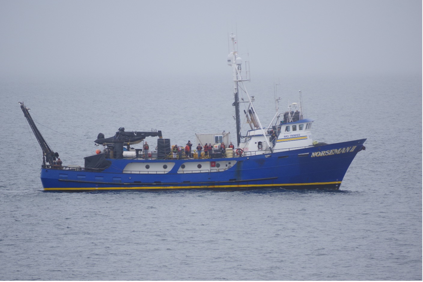
Figure 3. A picture of the Norseman II, the ship I was on in the Arctic, taken by the Japanese ship JAMSTEC on a short rendezvous between the Chukchi and Beaufort Seas.
By Rachel Kaplan, PhD student, OSU College of Earth, Ocean and Atmospheric Sciences and Department of Fisheries, Wildlife, & Conservation Sciences, Geospatial Ecology of Marine Megafauna Lab
Krill, a shrimplike crustacean found across our oceans, embodies the term “small but mighty”. Though individuals tend to be small, sometimes weighing in at less than a gram, the numerous species of krill have a global distribution and are estimated to collectively outweigh the entire human population. Much of my graduate research focuses on relationships between foraging whales and krill (Euphausia pacifica and Thysanoessa spinifera) in the Northern California Current (NCC) region. This work hinges on themes that are universal across environments: just as krill are ubiquitous across the global ocean, questions of prey quality, distribution, and ecological relationships with predators are universal.
Next week, I’m headed south to consider these questions in a very different foraging environment: the Western Antarctic Peninsula (WAP). One benefit of being a co-advised student is the incredible opportunity to be exposed to diverse projects and types of research. My graduate co-advisor, Kim Bernard, has studied krill in the WAP region for over a decade, and she is currently leading research into the implications of the shifting polar food web for Antarctic krill (Euphasia superba). Through a series of laboratory experiments and fieldwork, the project, titled “The Omnivore’s Dilemma: The effect of autumn diet on winter physiology and condition of juvenile Antarctic krill”, investigates the impact of climate-driven changes in diet on the health of juvenile krill in autumn and winter, a key time for their survival and recruitment. Winter is a poorly studied season in Antarctica, and this project has already shed light on the physiology, respiration, and growth potential of juvenile krill (Bernard et al., 2022).
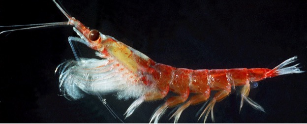
Figure 1: Antarctic krill are much bigger than those found in the NCC region – they can be as long as your thumb! (Source: Australian Antarctic Program)
Just as in the NCC region, krill are an essential link in Southern Ocean food webs, where they transfer energy from their microscopic prey to the higher trophic levels that eat them, including several species of fish, seals, penguins, and whales (Bernard & Steinberg, 2013; Cavan et al., 2019; Ducklow et al., 2013). These predators depend upon this high-quality prey to fuel their seasonal migrations and to build the energy reserves they need to survive the frigid Antarctic winter (Cade et al., 2022; Schaafsma et al., 2018). But, the quality of krill depends upon the food that it can consume itself, and climate change may alter their diet.
There’s a lot to love about krill, but my fascination with them is directly tied to their value as a food source for predators. I want to know how the caloric content of individuals and the aggregations they form changes spatially along the WAP, and how this might shift under climate-forced food web changes. This work will clarify the climate-driven variability in the quality of krill as prey, and the implications this might have for top predators in the region.
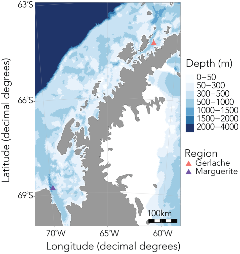
Figure 2: The upcoming field season will involve sampling krill along a latitudinal gradient in the WAP region, spanning approximately from the Gerlache Strait in the north to Marguerite Bay in the south (Bernard et al., 2022).
In order to investigate these questions, I’ll be spending the next six months based out of Palmer Station, the smallest of the United States’ research bases in Antarctica, along with Kim and our undergraduate intern Abby. During this upcoming field season, we’ll spend about a month at sea collecting krill samples and active acoustic data using an echosounder, and the rest of the time conducting experiments and sampling in the nearshore. Over the last year, Abby has worked with me to quantify krill caloric content in the NCC, as well as processing samples collected in Antarctica last year. I’m so impressed by everything she’s accomplished, and excited to see her take in this environment, learn a fresh set of experimental and field sampling approaches, and be inspired to ask new questions.
For me, heading south will be a bit like coming home. After graduating from college, I spent about nine months living at Palmer Station and working on the microbial ecology component of the long-term ecological research station there. The experience of being immersed in the WAP environment was foundational to my curiosity about ocean ecology and the impacts of climate change. It is also where I met Kim! All in all, this environment fueled my desire to study krill with Kim and spatial ecology with Leigh, and set me on the course I’m on today.
It also feels meaningful to return here again at this point in my educational journey. With new knowledge and questions I have formed while working in the NCC, I am now excited to apply this knowledge and consider similar questions in the WAP. Abby and I will write blogs through the season and post them here, so stay tuned for news from down south!
Figure 4: Kim and I (the two farthest right in the front row) prepare for a group costumed polar plunge in 2015. Will we do it again? We’ll keep you posted!
References
Bernard, K. S., & Steinberg, D. K. (2013). Krill biomass and aggregation structure in relation to tidal cycle in a penguin foraging region off the Western Antarctic Peninsula. ICES Journal of Marine Science, 70(4), 834–849. https://doi.org/10.1093/icesjms/fst088
Bernard, K. S., Steinke, K. B., & Fontana, J. M. (2022). Winter condition, physiology, and growth potential of juvenile Antarctic krill. Frontiers in Marine Science, 9, 990853. https://doi.org/10.3389/fmars.2022.990853
Cade, D. E., Kahane-Rapport, S. R., Wallis, B., Goldbogen, J. A., & Friedlaender, A. S. (2022). Evidence for Size-Selective Predation by Antarctic Humpback Whales. Frontiers in Marine Science, 9, 747788. https://doi.org/10.3389/fmars.2022.747788
Cavan, E. L., Belcher, A., Atkinson, A., Hill, S. L., Kawaguchi, S., McCormack, S., Meyer, B., Nicol, S., Ratnarajah, L., Schmidt, K., Steinberg, D. K., Tarling, G. A., & Boyd, P. W. (2019). The importance of Antarctic krill in biogeochemical cycles. Nat Commun, 10(1), 4742. https://doi.org/10.1038/s41467-019-12668-7
Ducklow, H., Fraser, W., Meredith, M., Stammerjohn, S., Doney, S., Martinson, D., Sailley, S., Schofield, O., Steinberg, D., Venables, H., & Amsler, C. (2013). West Antarctic Peninsula: An Ice-Dependent Coastal Marine Ecosystem in Transition. Oceanography, 26(3), 190–203. https://doi.org/10.5670/oceanog.2013.62
Schaafsma, F. L., Cherel, Y., Flores, H., van Franeker, J. A., Lea, M.-A., Raymond, B., & van de Putte, A. P. (2018). Review: The energetic value of zooplankton and nekton species of the Southern Ocean. Marine Biology, 165(8), 129. https://doi.org/10.1007/s00227-018-3386-z
It’s a tale as old as time: where there’s prey, there’ll be predators.
As apex predators, cetaceans act as top-down regulators of ecosystem function. While baleen whales act as “ecosystem engineers,” facilitating nutrient cycling in the ocean (Roman et al., 2014), toothed whales, or “odontocetes,” can impart keystone-level effects — that is, they disproportionately control the marine community’s food-web structure (Valls, Coll, & Christensen, 2015). The menus of prey vary widely by species — ranging from mircronekton to fish to squid – and by extension, vary widely across trophic levels.
So, it naturally follows the old adage: where there’s an abundance of prey, there’ll be an abundance of cetaceans. Yet, creating models that accurately depict this predator-prey relationship is, perhaps unsurprisingly, not as straightforward.
Detecting the ‘Predator’ Half of the Equation
Scientists have successfully documented cetacean presence drawing upon a myriad of methods, each bearing its unique advantages and limitations.
Visual surveys — spanning viewpoints from land, boats, and air — can attain precise spatial data and species ID. However, this data can be constrained by “availability bias” — that is, scientists can only observe cetaceans visible at the surface, not those obscured by the ocean’s depths. Species that spend less time near the surface are more likely to elude the observer’s line of sight, thereby being missed in the data. Consequently, visual surveys have historically undersampled deep-diving species. For instance, since its discovery by western science in 1945, the Hubb’s beaked whale (Mesoplodon carlshubbi) has only been observed alive twice by OSU MMI’s very own Bob Pitman, once in 1994 and another time in 2021.
Scientists have also been increasingly conducting acoustic surveys to document cetacean presence. Acoustic recorders can “hear” each cetacean species at different ranges. Baleen whales, which bellow low-frequency calls, can be heard as far as across ocean basins (Munk et al., 1994). Toothed whales whistle, echolocate, and buzz at frequencies so high they’re considered ultrasonic. But it comes at a trade-off: high-frequency sounds have shorter wavelengths, meaning they are heard across smaller ranges. This high variability, which scientists refer to as “detection range,” translates to not always knowing where the vocalizing cetacean that was recorded is: as such, acoustic data can lack the high-resolution spatial precision often achieved by visual surveys. Nevertheless, acoustic data triumphs in temporal extent, sometimes managing to record continuously at six months at a time. Additionally, animals can elude visual detection in poor weather conditions or if they have a cryptic surface expression, but detected in acoustic surveys (e.g., North Atlantic right whales (Eubalaena glacialis) (Ganley, Brault, & Mayo, 2019; Clark et. al, 2010). Thus, acoustic surveys may be especially optimal for recording elusive deep-dwellers that occupy the often rough Oregon waters, such as beaked whales, the focus of my research in collaboration with the GEMM Lab.
Prey can be measured by numerous methods. Most directly, prey can be measured “in-situ” — that is, prey is collected directly from the site where the cetaceans are detected or observed. A 2020 study combined fish trawls with a towed hydrophone array to identify which fish species odontocetes along the continental shelf of West Ireland (e.g., pilot whales, sperm whales, and Sowerby’s beaked whales) were feasting; the results found that odontocetes primarily fed upon mesopelagic fish and cephalopods (Breen et al., 2020). While trawls can glean species ID of prey, associating this prey data with depth and biomass can prove challenging.
Alternatively, prey can be detected via active acoustics. Echosounders release an acoustic signal that descends through the water column and then echoes back once it hits a sound-scattering organism. Beaked whales forage within deep scattering layers typically composed of myctophid fish and squid, both of which can echo back echosounder pings (Hazen et al., 2011). Thus, echosounder data can map prey density through the water column. When mapping prey density of beaked whales, Hazen et al. 2011 found a strong positive correlation among prey density, ocean vertical structure, and clicks primarily produced while foraging – suggesting beaked whales forage at depth when encountering large, multi-species aggregations of prey.
Most relevant to the HALO Project, prey is measured using proximate indices, which are more easily quantifiable metrics of ocean conditions, such as collected from ships via CTD casts or via satellite imagery, that are indirectly related to prey abundance. CTD data can provide information related to the water column structure, including depth and strength of the thermocline, depth of the mixed layer, depth of the euphotic zone, and total chlorophyll concentration in the euphotic zone (Redfern et al. 2006). Satellite imagery can characterize the dynamic patterns of the surface later, including sea surface temperature (SST), salinity, surface chlorophyll a, sea surface height (SSH), and sea surface currents (Virgili et al., 2022; Redfern et al., 2006). Ocean model data products can, such as the Regional Ocean Modeling System (ROMS) which models how an oceanic region of interest responds to physical processes, can provide water column variables related to eddy kinetic energy (EKE) and average temperature gradients (Virgili et al., 2022). In the case of my research with the HALO Project, we will be using oceanographic data collected through the Ocean Observatories Initiative to inform odontocete species distribution models.
Connecting the Dots: Linking Deep-Dwelling Top Predators and Prey
While scientists have made significant advances with collecting both cetacean and prey data, connecting the dots between the ecology of deep-dwelling odontocetes and the oceanographic parameters indicative of their prey still remains a challenge.
In the absence of in situ sampling, species distribution models of marine top predators often derive proxies for “prey data” from static bathymetric and dynamic surface water variables (Virgili et al., 2022). However, surface variables may be irrelevant to toothed whale prey inhabiting great depths (Virgili et al., 2022). Within the HALO Project, the deepest Rockhopper acoustic recording unit is recording odontocetes at nearly 3,000 m below the surface, putting into question the relevance of oceanographic parameters collected at the surface.
Figure 3: Schematic depicting the variation among different zones in the water column. Conditions at the surface may not represent conditions at depth. Credit: Barbara Ambrose, NOAA via NOAA Ocean Explorer.
In my research, I am setting out to estimate which oceanographic variables are optimal for explaining deep-dwelling odontocete presence. A 2022 study using visual survey data found that surface, subsurface, and static variables best explained beaked whale presence, whereas only surface and deep-water variables – not static – best explained sperm whale presence (Virgili et al., 2022). These results are associated with each species’ distinct foraging ecologies; beaked whales may truly only rely on organisms that live near the seabed, whereas sperm whales also feast upon meso-to-bathypelagic organisms, so they may be more sensitive to changes in water column conditions (Virgili et al., 2022). This study expanded the narrative: deep-water variables can also be key to predicting deep-dwelling odontocete presence. The oceanographic variables must be tailored to the ecology of each species of interest.
In the months ahead, I seek to build on this study by investigating which parameters best predict odontocete presence using an acoustic approach instead — I am looking forward to the results to come!
References
Breen, P., Pirotta, E., Allcock, L., Bennison, A., Boisseau, O., Bouch, P., Hearty, A., Jessopp, M., Kavanagh, A., Taite, M., & Rogan, E. (2020). Insights into the habitat of deep diving odontocetes around a canyon system in the northeast Atlantic ocean from a short multidisciplinary survey. Deep-Sea Research. Part I, Oceanographic Research Papers, 159, 103236. https://doi.org/10.1016/j.dsr.2020.103236
Clark, C.W., Brown, M.W., & Corkeron, P. (2010). Visual and acoustic surveys
for North Atlantic right whales, Eubalaena glacialis, in Cape Cod Bay, Massachusetts, 2001–2005: Management implications. Marine Mammal Science, 26(4), 837-854.
Ganley, L.C., Brault, S., & Mayo, C.A. (2019). What we see is not what there is: Estimating North Atlantic right whale Eubalaena glacialis local abundance. Endangered Species Research, 38, 101-113.
Hazen, E. L., Nowacek, D. P., St Laurent, L., Halpin, P. N., & Moretti, D. J. (2011). The relationship among oceanography, prey fields, and beaked whale foraging habitat in the Tongue of the Ocean. PloS One, 6(4), e19269–e19269.
Munk, W. H., Spindel, R. C., Baggeroer, A., & Birdsall, T. G. (1994). The Heard Island Feasibility Test. The Journal of the Acoustical Society of America, 96(4), 2330–2342. https://doi.org/10.1121/1.410105
Redfern, J. V., Ferguson, M. C., Becker, E. A., Hyrenbach, K. D., Good, C., Barlow, J., Kaschner, K., Baumgartner, M. F., Forney, K. A., Ballance, L. T., Fauchald, P., Halpin, P., Hamazaki, T., Pershing, A. J., Qian, S. S., Read, A., Reilly, S. B., Torres, L., & Werner, F. (2006). Techniques for cetacean–habitat modeling. Marine Ecology. Progress Series (Halstenbek), 310, 271–295.
Roman, J., Estes, J. A., Morissette, L., Smith, C., Costa, D., McCarthy, J., Nation, J., Nicol, S., Pershing, A., & Smetacek, V. (2014). Whales as marine ecosystem engineers. Frontiers in Ecology and the Environment, 12(7), 377–385.
Valls, A., Coll, M., & Christensen, V. (2015). Keystone species: toward an operational concept for marine biodiversity conservation. Ecological Monographs, 85(1), 29–47.
Virgili, A., Teillard, V., Dorémus, G., Dunn, T. E., Laran, S., Lewis, M., Louzao, M., Martínez-Cedeira, J., Pettex, E., Ruiz, L., Saavedra, C., Santos, M. B., Van Canneyt, O., Vázquez Bonales, J. A., & Ridoux, V. (2022). Deep ocean drivers better explain habitat preferences of sperm whales Physeter macrocephalus than beaked whales in the Bay of Biscay. Scientific Reports, 12(1), 9620–9620.
Predators have high energetic requirements that must be met to ensure reproductive success and population viability. For baleen whales, this task is particularly challenging since their foraging seasons are typically limited to short temporal windows during summer months when they migrate to productive high latitude environments. Foraging success is a balancing act whereby baleen whales must maximize the amount of energy they intake, while minimizing the amount of energy they expend to obtain food. Maximization of energy intake can be achieved by targeting the most beneficial prey. How beneficial a particular prey type (or prey patch) is can depend on a number of factors such as abundance, density, quality, size, and availability. Determining why baleen whales target particular prey types or patches is an important factor to enhance our understanding of their ecology and can ultimately aid in informing their management and conservation.
The GEMM Lab has several research projects in Newport and Port Orford, Oregon, on the Pacific Coast Feeding Group (PCFG), which is a sub-group of gray whales from the Eastern North Pacific (ENP) population. While ENP gray whales feed in the Bering, Chukchi, and Beaufort Seas (Arctic) in the summer months, the PCFG utilizes the range from northern California, USA to northern British Columbia, Canada. Our work to date has revealed a number of new findings about the PCFG including that they successfully gain weight during the summer on Oregon foraging grounds (Soledade Lemos et al. 2020). Furthermore, females that consistently use the PCFG range as their foraging grounds have successfully reproduced and given birth to calves (Calambokidis & Perez 2017). Yet, the abundance of the PCFG (~250 individuals; Calambokidis et al. 2017) is two orders of magnitude smaller than the ENP population (~20,000; Stewart & Weller 2021). So, why do more gray whales not use the PCFG range as their foraging grounds when it provides a shorter migration while also allowing whales to meet their high energetic requirements and ensure reproductive success? There are several hypotheses regarding this ecological mystery including that prey abundance, density, quality, and/or availability are higher in the Arctic than in the PCFG range, thus justifying the much larger number of gray whales that migrate further north for the summer feeding season.
Figure 1. Locations of prey samples collected with a light trap (open circles) or opportunistic collections of surface swarms of crab larvae (black triangles) in Newport, along the Oregon coast in the Pacific Northwest coast of the United States.
Our recent paper in Frontiers in Marine Science addressed the hypothesis that prey quality in the Arctic is higher than that of PCFG prey. To test this hypothesis, we first determined the quality (energetic value) of nearshore Oregon zooplankton species that PCFG gray whales are assumed to feed on (based on observations of fine-scale spatial and temporal overlap of foraging gray whales and sampled zooplankton). We obtained prey samples from nearshore reefs along the Oregon coast (Figure 1) as part of the GRANITE project using a light trap, which is a modified water jug with a weight and two floats attached to it, allowing the trap to sit approximately 1 meter above the seafloor. The trap contained a light which attracted zooplankton and effectively captured epibenthic prey of gray whales. Traps were left to soak overnight in locations where gray whales had been observed feeding extensively and collected the following morning. After identifying each specimen to species level and sorting them into reproductive stages, we used a bomb calorimeter to determine the caloric content of each species by month, year, and reproductive stage. We then compared these values to the literature-derived caloric value of the predominant benthic amphipod species that ENP gray whales feed on in the Arctic. These comparisons allowed us to extrapolate the caloric values gained from each prey type to estimated energetic requirements of pregnant and lactating female gray whales (Villegas-Amtmann et al. 2017).
Figure 2. Median caloric content and interquartile ranges by (A) species, (B) reproductive stage, and (C) month. Sizes of the zooplankton images are scaled at actual ratios relative to one another.
So, what did we find? Our sampling along the Oregon coast revealed six predominant zooplankton species: two mysid shrimp (Neomysis rayii, Holmesimysis sculpta), two amphipods (Atylus tridens, Polycheria osborni), and two types of crab larvae (Dungeness crab megalopae, porcelain crab larvae). These six Oregon prey species showed significant differences in their caloric values, with N. rayii and Dungeness crab megalopae having significantly higher calories per gram than the other prey species (Figure 2), though Dungeness crab megalopae stood out as the caloric gold mines for feeding gray whales in the PCFG range. Furthermore, month and reproductive stage also influenced the caloric content of some prey species, with gravid (aka pregnant) female mysid shrimp significantly increasing in calories throughout the summer (Figure 3).
Figure 3. Caloric content of different reproductive stages as a function of day of year (DOY; ranging from June to October) for the mysids Holmesimysis sculpta and Neomysis rayii, and the amphipod Atylus tridens. A. tridens is only represented on one panel due to small sample size of this species for the empty brood pouch and gravid reproductive stages. Asterisks indicate significant regressions (p<0.05).
The comparison of our Oregon prey caloric values to the predominant Arctic amphipod (Ampelisca macrocephala) proved our hypothesis wrong: Arctic amphipods do not have higher caloric value than Oregon prey, which would have help to explain why many more gray whales feed in the Arctic. We found that two Oregon prey species (N. rayii and Dungeness crab megalopae) have higher caloric values than A. macrocephala. If we translate the caloric contents of these prey to gray whale energetic needs, these differences mean that lactating and pregnant gray whales feeding in the PCFG area would need between 0.7-1.03 and 0.22-0.33 metric tons of prey less per day if they fed on Dungeness crab megalopae or N. rayii, respectively, than a whale feeding on Arctic A. macrocephala (Figure 4).
Figure 4. Daily prey requirements (A: metric tons; B: number of individuals) needed by pregnant and lactating female gray whales to meet their energetic requirements on the foraging ground. Energetic requirement estimates obtained from Villegas-Amtmann et al. (2017). Note the logarithmic scale of y-axis in panel (B).
If quality were the only prey metric that gray whales used to evaluate which food to eat, then it would make very little sense for so many gray whales to migrate to the Arctic when there are prey types of equal and greater quality available to them in the PCFG range. However, quality is not the only metric that influences gray whale foraging decisions. We therefore posit that the abundance, density, and availability of benthic amphipods in the Arctic are higher than the prey species found in the PCFG range. In fact, knowledge of the pulsed reproductive cycle of Dungeness and porcelain crabs allows us to conclude that the larvae of these two species are only available for a few weeks in the late spring and early summer on the Oregon coast. While mysid shrimp, such as N. rayii, are continuously available in the PCFG range throughout the summer, they may occur in less dense and more patchy aggregations than Arctic benthic amphipods. However, current estimates of prey density and abundance for either region are not available, and we do not have data on the energetic costs of the different foraging strategies. While there are still several unknowns, we have documented that higher prey quality in the Arctic is not the reason for the difference in gray whale foraging ground use in the eastern North Pacific.
References
Calambokidis, J., & Perez, A. 2017. Sightings and follow-up of mothers and calves in the PCFG and implications for internal recruitment. IWC Report SC/A17/GW/04 for the Workshop on the Status of North Pacific Gray Whales (La Jolla: IWC).
Calambokidis, J., Laake, J., & Perez, A. 2017. Updated analysis of abundance and population structure of seasonal gray whales in the Pacific Northwest, 1996-2015. IWC Report SC/A17/GW/05 for the Workshop on the Status of North Pacific Gray Whales (La Jolla: IWC).
Soledade Lemos, L., Burnett, J. D., Chandler, T. E., Sumich, J. L., & Torres, L. G. 2020. Intra- and inter-annual variation in gray whale body condition on a foraging ground. Ecosphere 11(4):e03094.
Stewart, J. D., & Weller, D. W. 2021. Abundance of eastern North Pacific gray whales 2019/2020. Department of Commerce, NOAA Technical Memorandum NMFS-SWFSC-639. United States: NOAA. doi:10.25923/bmam-pe91.
Villegas-Amtmann, S., Schwarz, L. K., Gailey, G., Sychenko, O., & Costa, D. P. 2017. East or west: the energetic cost of being a gray whale and the consequence of losing energy to disturbance. Endangered Species Research 34:167-183.
Fall has arrived in the Pacific Northwest. For humans, it means packing away the shorts and sandals, and getting the boots, raincoats and firewood ready. For gray whales, it means gulping down the last meal of zooplankton they will eat for several months and commencing the journey to warmer waters and sunnier skies in Mexico where they will spend the winter fasting, calving, and nursing. While the GEMM Lab may still squeeze in a day or two of field work this week, we are slowly wrapping up the 2020 field season as conditions get rougher and our beloved gray whales gradually depart our waters. This year marked the 6th year of data collection for both of our gray whale projects: the Newport project that investigates the impacts of multiple stressors on gray whale ecology and health, and the Port Orford project that explores fine-scale foraging ecology of gray whales and their zooplankton prey. Since it will be several months before the GEMM Lab heads back out onto the water again, I thought I would summarize our two field seasons, share some highlights, and muse about the drivers of our observations this summer.
Some snapshots of the field team hard at work this summer. Top left: Hunter Warwick operating the drone. Top right: PI Leigh Torres rocking the lab swag to protect against the sun. Bottom left: Lisa Hildebrand waiting for a whale to surface to get photos of it. Bottom right: Alejandro Fernandez Ajo transfers zooplankton from the light trap to sample jars.
Summaries
Our RHIB Ruby zipped around the central and southern Oregon coast on 33 different days. The summer started slow, with several days of field work where we encountered no whales despite surveying our entire study region. Our encounters picked up towards the end of June and by the end of the summer we totaled 107 sightings, encountering 46 unique individuals, 36 of which were resightings of known individuals we have identified in previous years. Our Newport star of the summer was Solé, a female gray whale we have seen every year since 2015, and we also saw many of our other regulars including Casper, Rafael, Spray, Bit, and Heart. None of these whales shone as bright as Solé though. We flew the drone over her 8 times and collected 7 fecal samples (one of which was the biggest whale fecal sample I have ever seen!). In total, we collected 30 fecal samples and flew the drone 88 times. These data will allow us to continue measuring body condition and hormone levels of Pacific Coast Feeding Group (PCFG) gray whales that use the Oregon coast.
Left: Our RHIB Ruby heading out for a day of field work in Port Orford, OR this summer. Right: Solé. Image captured under NOAA/NMFS permit #21678.
Our tandem research kayak Robustus may not be as zippy as Ruby (it is powered by human muscle rather than a powerful outboard engine after all), but it certainly continues to be a trusty vessel for the Port Orford team. The Port Orford research team, named the Theyodelers this year, collected 181 zooplankton samples and conducted 180 GoPro drops during the month of August from Robustus. Despite the many samples collected, the size of our prey samples remained relatively small throughout the whole season compared to previous years. The cliff team surveyed for a total of 117 hours, of which 15 were spent tracking whales with the theodolite and resulted in 40 different tracklines of whale movements. The whale situation in Port Orford was similar to the pattern of whale sightings in Newport, with low whale sightings at the start of the field season. Luckily, by the start of August (which marked the start of data collection for the Theyodelers), the number of whales using the Port Orford area, especially the two study sites, Mill Rocks & Tichenor Cove, had increased. Of the whales that came close enough to shore for us to identify using photo-id, we tracked 5 unique individuals, 3 of which we also saw in Newport this year. The Port Orford star of the summer was Smudge, with his tracklines making up a quarter of all of our tracklines collected. Smudge is also the whale we sighted most often last year in Port Orford.
Top: Theyodelers Mattea Holt Colberg and Liz Kelly sampling atop the kayak Robustus. Bottom: Smudge. Image captured under NOAA/NMFS permit #21678.
Highlights
Many of you may be familiar with the whale Scarlett (formally known as Scarback). Scarlett is a female, at least 24 years old (she was first documented in the PCFG range in 1996), who is well-known (and easily identified) by the large concave injury on her back that is covered in whale lice, or cyamids. No one knows for certain how Scarlett sustained this injury (though there are stories), however what we do know is that it has not prevented this female from reproducing and successfully raising several calves over her lifetime. The GEMM Lab last saw Scarlett with a calf (which we named Brown) in 2016. Since Scarlett is such a famous whale with a unique history, it shouldn’t be a surprise that one of our highlights this summer is the fact that Scarlett showed up with a new calf! In keeping with a “shades of red” theme, Leigh came up with the name Rose for the new calf. In July, the mom-calf pair put on quite a cute performance, with Rose rising up on Scarlett’s back, giving the team a glimpse of its face. The Scarlett-Rose highlight doesn’t end there though. Just last week, we had a very brief encounter in choppy, swelly waters with a small whale. The whale surfaced just twice allowing us to capture photo-id images, and as we were looking around to see where it would come up a third time, it suddenly breached approximately 20 m from the boat. Lo-and-behold, after comparing our photos of the whale to our catalogue, we realized that this elusive, breaching whale was Rose! I am excited to see whether Rose will return to the Oregon coast next summer and become a PCFG regular just like her mom.
Top: Scarlett, easily identified by the large concave injury on her back covered in cyamids. Bottom: Scarlett with her new calf Rose riding her back, giving us a glimpse of its face. Images captures under NOAA/NMFS permit #21678.
The highlight of the field season in Port Orford is the trial, failures and small successes of a new element to the project. There is still a lot that we do not know and understand about PCFG gray whales. One such thing is the way in which gray whales maneuver their large bodies in shallow rocky habitats, often riddled with kelp, and how exactly they capture their zooplankton prey in these environments. Using drones has certainly helped bring some light into this darkness and has led to the documentation of many novel foraging behaviors (Torres et al. 2018). However, the view from above is unable to provide the fine-scale interactions between whales, kelp, reefs, and zooplankton. Instead, we must somehow find a way to watch the whales underwater. Enter CamDo. CamDo is a technology company that designs specialty products to allow for GoPro cameras to be used for time-lapsed recordings over long periods of time in harsh environmental conditions. One of their products is a housing specifically designed for long-term filming underwater – exactly what we need! The journey was not as easy as simply purchasing the housing. We also needed to build a lander for the housing to sit on (thankfully our very own Todd Chandler designed and built something for us), and coordinate with divers and a vessel to deploy and retrieve the set-up, as well as undertake weekly battery and SD cards swaps (thankfully Dave Lacey of South Coast Tours and a very generous group of divers* donated their time and resources to make this happen). We unfortunately had some technological difficulties and bad visibility for the first 4 weeks (precisely why this CamDo effort was a pilot season this year), however we had some small success in the last 2 weeks of deployment that give us hope for the future. The camera recorded a lot of things: thick layers of mysids, countless rockfish and lingcod, several swimming and foraging murres, a handful of harbor seals, and two encounters of the species we were hoping to film – gray whales! While the footage is not the ‘money shot’ we are hoping to film (aka, a headstanding gray whale eating zooplankton right in front of the camera), the fact that we captured gray whales in the first place has showed us that this set-up is a promising investment of time, money and effort that will hopefully deliver next year.
Top left: CamDo atop its lander designed and built by Todd Chandler. Top right: Divers getting ready to get into the water for a battery and SD card swap. Bottom: Dave Lacey and two of our divers with the Black Pearl, South Coast Tour’s boat.
Musings
You may have picked up on the fact that we had slow starts to our field seasons in both Newport and Port Orford. Furthermore, while the number of whale sightings did increase in both locations throughout the field seasons, the number of sightings and whales per day were lower than they have been in previous years. For example, in 2018, we identified 15 different individuals in the month of August in Port Orford (compared to just 5 this year). In 2019, 63 unique whales were seen in Newport (compared to 46 this year). Interestingly, we had a greater diversity of encountered individuals at the start and end of the season in Newport, with a relatively small number of different individuals in July and August. While I cannot provide a definitive reason (or reasons) as to why patterns were observed (we will need to analyze several years of our data to try and understand why), I have some hypotheses I wish to share with you.
As I mentioned in a previous blog, this summer the coastal upwelling along the Oregon coast was delayed (Figure 1). Typically, peak upwelling occurs during the month of June or shortly thereafter, bringing nutrient-rich, deep waters to the surface and, when mixed with sunlight, a lot of productivity. This productivity sets off a chain of reactions — the input of nutrients leads to increased phytoplankton production, which in turn leads to increased zooplankton production, resulting in growth and development of larger organisms that consume zooplankton, such as rockfish and gray whales. If the timing of upwelling is delayed, then so too is this chain of reactions. As you can see from Figure 1, the red lines show that the peak upwelling this year occurred far later in the summer than any year in the last 10 years, with the exception of 2012. Gray whales may have cued into this delay and therefore also delayed their arrival to the PCFG feeding grounds, hence causing us to have low sighting rates at the start of our season. However, this is mostly speculative as we still do not understand the functional mechanisms by which cetaceans, such as gray whales, detect prey across different scales, and to what extent oceanographic conditions like upwelling may play a role in prey availability (Torres 2017).
Figure 1. 10 year time series of the Coastal Upwelling Transport Index (CUTI). CUTI represents the amount of upwelling (positive numbers) or downwelling (negative numbers). The light-colored lines representthe CUTI at that point in time while the dark, bold line represents the long-term average.The vertical red lines represent the point of peak upwelling in that summer and the horizontal green line shows the peak level of upwelling in 2020 relative to all previous years.
Furthermore, the green line in Figure 1shows that even after peak upwelling was reached this year, upwelling conditions were lower than all the other peaks in the previous 10 years. We know that weak upwelling is correlated to poor body condition of PCFG gray whales in subsequent years (Soledade Lemos et al. 2020). Upon arriving to the Oregon coast feeding grounds, gray whales may have noticed that it was shaping up to be a poor prey year (we certainly noticed it in Port Orford in the emptiness of our zooplankton net). Faced with this low resource availability, individuals had to make important decisions – risk staying in a currently prey-poor environment or continue the journey onward, searching for better prey conditions elsewhere. This conundrum is known as the marginal value theorem, whereby an individual must decide whether it should abandon the patch it is currently foraging on and move on to search for a new patch without knowing how far away the next patch may be or its value relative to the current patch (Charnov 1976). If we think of the Oregon coast as the ‘current patch’, then we can see how the marginal value theorem translates to the situation gray whales may have found themselves in at the start of the summer.
Yet, an individual gray whale does not make these decisions in a vacuum. Instead, all gray whales in the same area are faced with the same conundrum. Seminal work by Pianka (1974) showed that when resources, such as food, are abundant, then competition between predators is low because there is enough food to go around. However, when resources dwindle, competition increases and the niches of predators begin to overlap more and more. With Charnov and Pianka’s theories in mind, we can see two groups of gray whales emerge from our 2020 field work observations: those that stayed in the ‘current patch’ (Oregon) and those that decided to seek out a new patch in hopes that it would be a better one. Solé certainly belongs in the first group. We saw her consistently throughout the whole summer. In fact, she was oftentimes so predictable that we would find her foraging on the same reef complex every time we went out to survey. Smudge may also belong in this group, however it is hard to say definitively since we only survey in Port Orford in late July and August. In contrast, I would place whales such as Spray and Heart in the second group since we saw them early in the summer and then not again until mid-to-late September. Where did they go in the interim? Did they go somewhere else in the PCFG range? Or did they venture all the way up to Alaska to the primary Eastern North Pacific (ENP) gray whale feeding grounds? Did their choice to search for food elsewhere pay off?
As I said earlier, these are all just musings for now, but the GEMM Lab is already hard at work trying to answer these questions. Stay tuned to see what we find!
* Thanks to all the divers who assisted with the pilot CamDo season: Aaron Galloway, Ross Whippo, Svetlana Maslakova, Taylor Eaton, Cori Kane, Austin Williams, Justin Smith
References
Charnov, E.L. 1976. Optimal Foraging, the Marginal Value Theorem. Theoretical Population Biology 9(2):129-136.
Pianka, E.R. 1974. Niche Overlap and Diffuse Competition. PNAS 71(5):2141-2145.
Soledade Lemos, L., Burnett, J.D., Chandler, T.E., Sumich, J.L., and L.G. Torres. 2020. Intra- and inter-annual variation in gray whale body condition on a foraging ground. Ecosphere 11(4):e03094.
Torres, L.G. 2017. A sense of scale: Foraging cetaceans’ use of scale-dependent multimodal sensory systems. Marine Mammal Science 33(4):1170-1193.
Torres, L.G., Nieukirk, S.L., Lemos, L., and T.E. Chandler. 2018. Drone Up! Quantifying Whale Behavior From a New Perspective Improves Observational Capacity. Frontiers in Marine Science: https://doi.org/10.3389/fmars.2018.00319.
When humans count calories it is typically to regulate and limit calorie intake. What I am wondering about is whether gray whales are aware of caloric differences in the prey that is available to them and whether they make foraging decisions based on those differences. In last week’s post, Dawn discussed what makes a good meal for a hungry blue whale. She discussed that total prey biomass of a patch, as well as how densely aggregated that patch is, are the important factors when a blue whale is picking its next meal. If these factors are important for blue whales, is it same for gray whales? Why even consider the caloric value of their prey?
Gray and blue whales are different in many ways; one way is that blue whales are krill specialists whereas gray whales are more flexible foragers. The Pacific Coast Feeding Group (PCFG) of gray whales in particular are known to pursue a more varied menu. Previous studies along the PCFG range have documented gray whales feeding on mysid shrimp (Darling et al. 1998;Newell 2009), amphipods (Oliver et al. 1984; Darling et al. 1998), cumacean shrimp (Jenkinson 2001; Moore et al. 2007;Gosho et al. 2011), and porcelain crab larvae (Dunham and Duffus 2002), to name a few. Based on our observations in the field and from our drone footage, we have observed gray whales feeding on reefs (likely on mysid shrimp), benthically (likely on burrowing amphipods), and at the surface on crab larvae (Fig. 1). Therefore, while both blue and PCFG whales must make decisions about prey patch quality based on biomass and density of the prey, gray whales have an extra decision to make based on prey type since their prey menu items occupy different habitats that require different feeding tactics and amount of energy to acquire them. In light of these reasons, I hypothesize that prey caloric value factors into their decision of prey patch selection.
Figure 1. Gray whales use several feeding tactics to obtain a variety of coastal Oregon zooplankton prey including jaw snapping (0:12 of video), drooling mud (0:21), and head standing (0:32), to name a few.
This prey selection process is crucial since PCFG gray whales only have about 6 months to consume all the food they need to migrate and reproduce (even less for the Eastern North Pacific (ENP) gray whales since their journey to their Arctic feeding grounds is much longer). You may be asking, well if feeding is so important to gray whales, then why not eat everything they come across? Surely, if they ate every prey item they swam by, then they would be fine. The reason it isn’t quite this simple is because there are energetic costs to travel to, search for, and consume food. If an individual whale simply eats what is closest (a small, poor-quality prey patch) and uses up more energy than it gains, it may be missing out on a much more beneficial and rewarding prey patch that is a little further away (that patch may disperse or another whale may eat it by the time this whale gets there). Scientists have pondered this decision-making process in predators for a long time. These ponderances are best summed up by two central theories: the optimal foraging theory (MacArthur & Pianka 1966) and the marginal value theorem (Charnov 1976). If you are a frequent reader of the blog, you have probably heard these terms once or twice before as a lot of the questions we ask in the GEMM Lab can be traced back to these concepts.
Optimal foraging theory (OFT) states that a predator should pick the most beneficial resource for the lowest cost, thereby maximizing the net energy gained. So, a gray whale should pick a prey patch where it knows that it will gain more energy from consuming the prey in the patch than it will lose energy in the process of searching for and feeding on it. Marginal value theorem elaborates on this OFT concept by adding that the predator also needs to consider the cost of giving up a prey patch to search for a new one, which may or may not end up being more profitable or which may take a very long time to find (and therefore cost more energy).
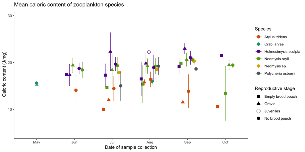
The second chapter of my thesis will investigate whether individual gray whales have foraging preferences by relating feeding location to prey quality (community composition) and quantity (relative density). However, in order to do that, I first must know about the quality of the individual prey species, which is why my first chapter explores the caloric content of common coastal zooplankton species in Oregon that may serve as gray whale prey. The lab work and analysis for that chapter are completed and I am in the process of writing it up for publication. Preliminary results (Fig. 2) show variation in caloric content between species (represented by different colors) and reproductive stages (represented by different shapes), with a potential increasing trend throughout the summer. These results suggest that some species and reproductive stages may be less profitable than others based solely on caloric content.
Figure 2. Mean caloric content (J/mg) of coastal Oregon zooplankton (error bars represent standard deviation) from May-October in 2017-2018. Colors represent species and shapes represent reproductive stage.
Now that we have established that there may be bigger benefits to feeding on some species over others, we have to consider the availability of these zooplankton species to PCFG whales. Availability can be thought of in two ways: 1) is the prey species present and at high enough densities to make searching and foraging profitable, and 2) is the prey species in a habitat or depth that is accessible to the whale at a reasonable energetic cost? Some prey species, such as crab larvae, are not available at all times of the summer. Their reproductive cycles are pulsed (Roegner et al. 2007) and therefore these prey species are less available than species, such as mysid shrimp, that have more continuous reproduction (Mauchline 1980). Mysid shrimp appear to seek refuge on reefs in rock crevices and among kelp, whereas amphipods often burrow in soft sediment. Both of these habitat types present different challenges and energetic costs to a foraging gray whale; it may take more time and energy to dislodge mysids from a reef, but the payout will be bigger in terms of caloric gain than if the whale decides to sift through soft sediment on the seafloor to feed on amphipods. This benthic feeding tactic may potentially be a less costly foraging tactic for PCFG whales, but the reward is a less profitable prey item.
My first chapter will extend our findings on the caloric content of Oregon coastal zooplankton to facilitate a comparison to the caloric values of the main ampeliscid amphipod prey of ENP gray whales feeding in the Arctic. Through this comparison I hope to assess the trade-offs of being a PCFG whale rather than an ENP whale that completes the full migration cycle to the primary summer feeding grounds in the Arctic.
References
Charnov, E. L. 1976. Optimal foraging: the marginal value theorem. Theoretical Population Biology 9:129-136.
Darling, J. D., Keogh, K. E. and T. E. Steeves. 1998. Gray whale (Eschrichtius robustus) habitat utilization and prey species off Vancouver Island, B.C. Marine Mammal Science 14(4):692-720.
Dunham, J. S. and D. A. Duffus. 2002. Diet of gray whales (Eschrichtius robustus) in Clayoquot Sound, British Columbia, Canada. Marine Mammal Science 18(2):419-437.
Gosho, M., Gearin, P. J., Jenkinson, R. S., Laake, J. L., Mazzuca, L., Kubiak, D., Calambokidis, J. C., Megill, W. M., Gisborne, B., Goley, D., Tombach, C., Darling, J. D. and V. Deecke. 2011. SC/M11/AWMP2 submitted to International Whaling Commission Scientific Committee.
Jenkinson, R. S. 2001. Gray whale (Eschrichtius robustus) prey availability and feeding ecology in Northern California, 1999-2000. Master’s thesis, Humboldt State University.
MacArthur, R. H., and E. R. Pianka. 1966. On optimal use of a patchy environment. American Naturalist 100:603-609.
Mauchline, J. 1980. The larvae and reproduction in Blaxter, J. H. S., Russell, F. S., and M. Yonge, eds. Advances in Marine Biology vol. 18. Academic Press, London.
Moore, S. E., Wynne, K. M., Kinney, J. C., and C. M. Grebmeier. 2007. Gray whale occurrence and forage southeast of Kodiak Island, Alaska. Marine Mammal Science 23(2)419-428.
Newell, C. L. 2009. Ecological interrelationships between summer resident gray whales (Eschrichtius robustus) and their prey, mysid shrimp (Holmesimysis sculpta and Neomysis rayii) along the central Oregon coast. Master’s thesis, Oregon State University.
Oliver, J. S., Slattery, P. N., Silberstein, M. A., and E. F. O’Connor. 1984. Gray whale feeding on dense ampeliscid amphipod communities near Bamfield, British Columbia. Canadian Journal of Zoology 62:41-49.
Roegner, G. C., Armstrong, D. A., and A. L. Shanks. 2007. Wind and tidal influences on larval crab recruitment to an Oregon estuary. Marine Ecology Progress Series 351:177-188.
Knowing what and how much prey a predator feeds on are key components to better understanding and conserving that predator. Prey abundance and availability are frequently predictors for marine predator reproductive success and population dynamics. It is the reason why the GEMM Lab makes a concerted effort to not only track our main taxa of interest (marine mammals) but to simultaneously measure their prey. However, over the last decade or two, there has been increased recognition that prey quality is also highly important in understanding a predator’s ecology (Spitz et al. 2012). Optimal foraging theory is a widely accepted framework that posits that predators should attempt to maximize energy gained and minimize energy spent during a foraging event (Charnov 1976, Krebs 1978, Pyke 1984). Thus, knowledge of how valuable a prey item is in terms of its energetic content is an important part of the equation when applying optimal foraging theory to a predator of interest.
Ideally, the prey species with the highest energetic value would also be the easiest, most ubiquitous and least energetically expensive prey item to capture and consume, such that a predator truly could expend very little energy to get very high energetic rewards. However, it rarely is this straightforward. The caloric content of several marine prey species has been shown to increase with increasing size (e.g. Benoit-Bird 2004; Fig. 1), both length and weight. Yet, increasing size often also means increased mobility and, as a result, ability to evade and escape predation. Furthermore, increasing size also inherently means decreasing abundances – there will always be billions more krill in the ocean than whales based solely on cost of reproduction. Therefore, just based on sheer numbers, there are fewer big prey items, which increases the time between, and decreases the likelihood of, a predator encountering big prey items. So, there are clear trade-offs here. It may take longer to locate and capture a high value prey item, which costs more energy to capture, but the payout could potentially be much bigger. However, if a predator gambles too much, then their net energy expenditure to obtain high value prey may be higher than the net energy gained. Instead, it may be worth pursuing smaller prey items with lower energetic values, where discovery and capture success are higher and more frequent. However, in this case, many, many more pursuits are likely needed, thus costing more energy to meet daily energetic demands.
Figure 1. Increasing caloric content with increasing length (a) and wet weight (b). Figures and caption reproduced from Benoit-Bird 2004.
Is your head spinning as much as mine? Let me try and simplify this complex web of interactions with a tangible example. Bowen et al. (2002) investigated foraging of harbor seals in Nova Scotia to assess prey profitability of different species. By attaching camera systems to the backs of 39 adult male harbor seals, the authors identified sand lance and flounder to be the most targeted prey species. However, there were significant differences in pursuit/handling cost per prey type (kJ/min) with sand lance only requiring 14.8 ± 2.7, whereas flounder required significantly more at 30.3 ± 7.9. Therefore, based solely on energy required to capture prey, the sand lance would seem to be the better option. In fact, to a certain degree, this hypothesis is actually true when we compare the energetic content of the two prey types. Sand lance have a higher energetic value at lengths of 10 and 15 cm (53.6 and 95.8 kJ, respectively) compared to flounder (22.6 and 88.6 kJ, respectively). So, the net gain of a harbor seal foraging on a 15 cm sand lance (assuming that it only takes 1 minute to catch the fish – this is more for explanatory purposes as it likely takes much longer for a harbor seal to capture a fish) would be 81 kJ. This gain is larger than that of a 15 cm flounder (58.3 kJ). However, once we compare these fish at 20 and 25 cm lengths, the flounder actually becomes the more beneficial prey item at 232.6 and 492.3 kJ, respectively, over the sand lance (158.1 and 233.8 kJ). Now, assuming once again that it only takes 1 minute to catch the fish, the harbor seal enjoys a net energetic gain of a whopping 462 kJ when capturing a 25 cm flounder compared to 219 kJ for a sand lance of the same size – that makes the flounder more than twice as profitable!
The Bowen et al. study is an excellent demonstration of the importance of considering the quality of prey items when studying the ecology of marine predators. However, the authors did not assess the relative availability of sand lance and flounder. Ideally, foraging ecology studies aimed at understanding prey choice would try to address both important prey metrics – quality and quantity. This goal is the exact aim of my second Master’s thesis chapter where I am investigating whether prey quality (determined through community composition and caloric content) or prey quantity (measured as relative density) is more important in driving fine-scale gray whale foraging behavior in Port Orford, Oregon (Fig. 2). This question can be simplified by asking does it matter more what prey is in an area, or how much prey there is in an area? Or we can relate it back to the title of this post by asking whether individual gray whales would rather attend a cheap all-you-can-eat buffet or an expensive fine-dining restaurant. I am unfortunately not quite done with my analyses yet (but I’m getting closer!) and therefore am not ready to answer these questions. However, I have done extensive research on this topic and therefore am in a position to briefly mention a few other studies that have investigated these questions for other marine predators.
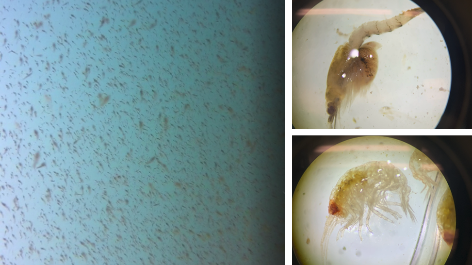
Figure 2. A question of what or how much. Left image: example of the screenshots we take to estimate relative prey density in Port Orford. Right images: two examples of the main prey species we find (top: mysid shrimp Neomysis rayii with a full brood pouch; bottom: amphipod Polycheria osborni).
Ludynia et al. (2010) explored reasons why African penguin (Spehniscus demersus) numbers have declined in Namibia. They found that after the collapse of pelagic fish stocks in the 1970s (including the principal penguin prey item, sardine), African penguins switched to feeding on bearded goby, which are considered a low-energy prey species. Bearded goby are relatively abundant along Namibia’s southern coast and as such, limited prey availability is not the reason for declining African penguin numbers. Therefore, the authors concluded that the low quality of bearded goby (compared to sardine) appears to be the reason for declining population trends of the penguins. This study demonstrates that African penguins do better when eating at a fine-dining restaurant, rather than loading up a whole plate of junk food.
Grémillet et al. (2004) studied the foraging effort and number of successful prey captures per foraging trip (yield) of great cormorants (Phalacrocorax carbo) in Greenland in relation to prey abundance and quality within their foraging areas. The authors radio-tracked 11 great cormorants during a total of 163 foraging trips to estimate foraging effort and yield. The study found that contrary to the authors’ hypothesis, great cormorants foraged in areas of low prey abundance where the average caloric value was also relatively low. Therefore, in this example, it would seem that the predator of interest prioritizes neither high quality nor quantity when foraging.
Haug et al. (2002) investigated the variations in minke whale (Balaenoptera acutorostrata) diet and body condition in response to ecosystem changes in the Barents Sea. The main prey item of minke whales in the Barents Sea is immature herring. However, when recruitment failure and subsequent weak cohorts leads to reduced availability of immature herring, minke whales switched their diet to other prey items such as krill, capelin, and sometimes other gadoid fish species. The authors found a correlation between body condition of minke whales and immature herring abundances, such that minke whales displayed a poor body condition during low immature herring abundances. However, in the years of low immature herring abundance, abundances of krill and capelin were not low. Therefore, similar to the Ludynia et al. (2010) study, it seems that minke whales in the Barents Sea also do better in years when the prey type of highest caloric value is the most abundant. However, decreases in high quality prey has not led to population declines in minke whales in the Barents Sea, indicating that they likely take advantage of high quantities of low quality prey, unlike the African penguins.
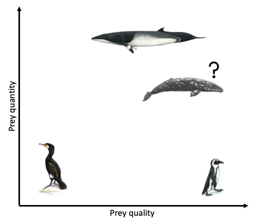
Clearly, the answer as to whether marine predators prefer quality over quantity is not simple and constant. Rather, prey preference varies based on predator needs and ecology, falling anywhere on a broad spectrum from low to high prey quality and low to high prey quantity (Fig. 3). To a certain extent, it probably also is not solely predator choice that determines what they eat but many other factors, such as climate, disturbance, and health. As a result, these preferences and choices will likely be fluid, rather than fixed. While I anticipate that individual gray whales will be flexible foragers, I do hypothesize that when there is a prey patch of a higher energetic value in the area, whales will preferentially consume these patches over areas where there is less energetically rich prey, even if it is more abundant.
Figure 3. A spectrum of prey quantity and quality. Giant cormorants forage on low prey quality & quantity (Grémillet et al. 2004). African penguin populations are declining despite high abundances of low quality prey, suggesting that high prey quality is important for their survival (Ludynia et al. 2010). Body condition of Barents Sea minke whales decreases when high quality prey is less abundant, however their populations have not declined, suggesting they instead exploit high abundances of low quality prey (Haug et al. 2002). What will the gray whales do?
Literature cited
Benoit-Bird, K. J. 2004. Prey caloric value and predator energy needs: foraging predictions for wild spinner dolphins. Marine Biology 145:435-444.
Bowen, W. D., D. Tuley, D. J. Boness, B. M. Bulheier, and G. J. Marshall. 2002. Prey-dependent foraging tactics and prey profitability in a marine mammal. Marine Ecology Progress Series 244:235-245.
Charnov, E. L. 1976. Optimal foraging, the marginal value theorem. Theoretical Population Biology 9(2):129-136.
Grémillet D., G. Kuntz, F. Delbart, M. Mellet, A. Kato, J-P. Robin, P-E. Chaillon, J-P. Gendner, S-H. Lorentsen, and Y. Le Maho. 2004. Linking the foraging performance of a marine predator to local prey abundance. Functional Ecology 18(6):793-801.
Haug, T., U. Lindstrøm, and K. T. Nilssen. 2002. Variations in minke whale (Balaenoptera acutorostrata) diet and body condition in response to ecosystem changes in the Barents Sea. Sarsia 87(6):409-422.
Krebs, J. R. 1978. Optimal foraging: decision rules for predators. Behvaioral Ecology: An Evolutionary Approach, eds. Krebs, J. R., and N. B. Davies. Oxford: Blackwell.
Ludynia, J., J-P. Roux, R. Jones, J. Kemper, and L. G. Underhill. 2010. Surviving off junk: low-energy prey dominates the diet of African penguins Spheniscus demersus at Mercury Island, Namibia, between 1996 and 2009. African Journal of Marine Science 32(3):563-572.
Pyke, G. H. 1984. Optimal foraging theory: a critical review. Annual Reviews of Ecology and Systematics 15:523-575.
Spitz, J., A. W. Trites, V. Becquet, A. Brind’Amour, Y. Cherel, R. Galois, and V. Ridoux. 2012. Cost of living dictates what whales, dolphins and porpoises eat: the importance of prey quality on predator foraging strategies. PLoS ONE 7(11):e50096.
Young, J. K., B. A. Black, J. T. Clarke, S. V. Schonberg, and K. H. Dunton. 2017. Abundance, biomass and caloric content of Chukchi Sea bivalves and association with Pacific walrus (Odobenus rosmarus divergens) relative density and distribution in the northeastern Chukchi Sea. Deep-Sea Research Part II 144:125-141.
The last two months have been challenging for everyone across the world. While I have also experienced lows and disappointments during this time, I always try to see the positives and to appreciate the good things every day, even if they are small. One thing that I have been extremely grateful and excited about every week is when the clock strikes 9:58 am every Thursday. At that time, I click a Zoom link and after a few seconds of waiting, I am greeted by the smiling faces of the GEMM Lab. This spring term, our Principal Investigator Dr. Leigh Torres is teaching a reading and conference class entitled ‘Cetacean Behavioral Ecology’. Every week there are 2-3 readings (a mix of book chapters and scientific papers) focused on a particular aspect of behavioral ecology in cetaceans. During the first week we took a deep dive into the foundations of behavioral ecology (much of which is terrestrial-based) and we have now transitioned into applying the theories to more cetacean-centric literature, with a different branch of behavior and ecology addressed each week.
Leigh dedicated four weeks of the class to discussing foraging behavior, which is particularly relevant (and exciting) to me since my Master’s thesis focuses on the fine-scale foraging ecology of gray whales. Trying to understand the foraging behavior of cetaceans is not an easy feat since there are so many variables that influence the decisions made by an individual on where and when to forage, and what to forage on. While we can attempt to measure these variables (e.g., prey, environment, disturbance, competition, an individual’s health), it is almost impossible to quantify all of them at the same time while also tracking the behavior of the individual of interest. Time, money, and unworkable weather conditions are the typical culprits of making such work difficult. However, on top of these barriers is the added complication of scale. We still know so little about the scales at which cetaceans operate on, or, more importantly, the scales at which the aforementioned variables have an effect on and drive the behavior of cetaceans. For instance, does it matter if a predator is 10 km away, or just when it is 1 km away? Is a whale able to sense a patch of prey 100 m away, or just 10 m away? The same questions can be asked in terms of temporal scale too.
What is that gray whale doing in the kelp? Source: F. Sullivan.
As such, cetacean field work will always involve some compromise in data collection between these factors. A project might address cetacean movements across large swaths of the ocean (e.g., the entire U.S. west coast) to locate foraging hotspots, but it would be logistically complicated to simultaneously collect data on prey distribution and abundance, disturbance and competitors across this same scale at the same time. Alternatively, a project could focus on a small, fixed area, making simultaneous measurements of multiple variables more feasible, but this means that only individuals using the study area are studied. My field work in Port Orford falls into the latter category. The project is unique in that we have high-resolution data on prey (zooplankton) and predators (gray whales), and that these datasets have high spatial and temporal overlap (collected at nearly the same time and place). However, once a whale leaves the study area, I do not know where it goes and what it does once it leaves. As I said, it is a game of compromises and trade-offs.
Ironically, the species and systems that we study also live a life of compromises and trade-offs. In one of this week’s readings, Mridula Srinivasan very eloquently starts her chapter entitled ‘Predator/Prey Decisions and the Ecology of Fear’ in Bernd Würsig’s ‘Ethology and Behavioral Ecology of Odontocetes’ with the following two sentences: “Animal behaviors are governed by the intrinsic need to survive and reproduce. Even when sophisticated predators and prey are involved, these tenets of behavioral ecology hold.”. Every day, animals must walk the tightrope of finding and consuming enough food to survive and ensure a level of fitness required to reproduce, while concurrently making sure that they do not fall prey to a predator themselves. Krebs & Davies (2012) very ingeniously use the idea of economic analysis of costs and benefits to understand foraging behavior (but also behavior in general). While foraging, individuals not only have to assess potential risk (Fig. 1) but also decide whether a certain prey patch or item is profitable enough to invest energy into obtaining it (Fig. 2).
Leigh’s class has been great, not only to learn about foundational theories but to then also apply them to each of our study species and systems. It has been exciting to construct hypotheses based on the readings and then dissect them as a group. As an example, Sih’s 1984 paper on the behavioral response race of predators and prey prompted a discussion on responses of predators and prey to one another and how this affects their spatial distributions. Sih posits that since predators target areas with high prey densities, and prey will therefore avoid areas that predators frequent, their responses are in conflict with one another. Resultantly, there will be different outcomes depending on whichever response dominates. If the predator’s response dominates (i.e. predators are able to seek out areas of high prey density before prey can respond), then predators and prey will have positively correlated spatial distributions. However, if the prey responses dominate, then the spatial distributions of the two should be negatively correlated, as predators will essentially always be ‘one step behind’ the prey. Movement is most often the determinant factor to describe the strength of these relationships.
Video 1. Zooplankton closest to the camera will jump or dart away from it. Source: GEMM Lab.
So, let us think about this for gray whales and their zooplankton prey. The latter are relatively immobile. Even though they dart around in the water column (I have seen them ‘jump’ away from the GoPro when we lower it from the kayak on several occasions; Video 1), they do not have the ability to maneuver away fast or far enough to evade a gray whale predator moving much faster. As such, the predator response will most likely always be the strongest since gray whales operate at a scale that is several orders of magnitude greater than the zooplankton. However, the zooplankton may not be as helpless as I have made them seem. Based on our field observations, it seems that zooplankton often aggregate beneath or around kelp. This behavior could potentially be an attempt to evade predators as the kelp and reef crevices may serve as a refuge. So, in areas with a lot of refuges, the prey response may in fact dominate the relationship between gray whales and zooplankton. This example demonstrates the importance of habitat in shaping predator-prey interactions and behavior. However, we have often observed gray whales perform “bubble blasts” in or near kelp (Video 2). We hypothesize that this behavior could be a foraging tactic to tip the see-saw of predator-prey response strength back into their favor. If this is the case, then I would imagine that gray whales must decide whether the energetic benefit of eating zooplankton hidden in kelp refuges outweighs the energy required to pursue them (Fig. 2). On top of all these choices, are the potential risks and threats of boat traffic, fishing gear, noise, and potential killer whale predation (Fig. 1). Bringing us back to the analogy of economic analysis of costs and benefits to predator-prey relationships. I never realized it so clearly before, but gray whales sure do have a lot of decisions to make in a day!
Video 2. Drone footage of a gray whale foraging in kelp and performing a “bubble blast” at 00:40. Footage captured under NMFS permit #21678. Source: GEMM Lab.
Trying to tease apart these nuanced dynamics is not easy when I am unable to simply ask my study subjects (gray whales) why they decided to abandon a patch of zooplankton (Were the zooplankton too hard to obtain because they sought refuge in kelp, or was the patch unprofitable because there were too few or the wrong kind of zooplankton?). Or, why do gray whales in Oregon risk foraging in such nearshore coastal reefs where there is high boat traffic (Does their need for food near the reefs outweigh this risk, or do they not perceive the boats as a risk?). So, instead, we must set up specific hypotheses and use these to construct a thought-out and informed study design to best answer our questions (Mann 2000). For the past few weeks, I have spent a lot of time familiarizing myself with spatial packages and functions in R to start investigating the relationships between zooplankton and kelp hidden in the data we have collected over 4 years, to ultimately relate these patterns to gray whale foraging. I still have a long and steep journey before I reach the peak but once I do, I hope to have answers to some of the questions that the Cetacean Behavioral Ecology class has inspired.
Literature cited
Krebs, J. R., and N. B. Davies. 2012. Economic decisions and the individual in Davies, N. B. et al., eds. An introduction to behavioral ecology. John Wiley & Sons, Oxford.
Mann, J. 2000. Unraveling the dynamics of social life: long-term studies and observational methods in Mann, J., ed. Cetacean societies: field studies of dolphins and whales. University of Chicago Press, Chicago.
Sih, A. 1984. The behavioral response race between predator and prey. The American Naturalist 123:143-150.
Srinivasan, M. 2019. Predator/prey decisions and the ecology of fear in Würsig, B., ed. Ethology and ecology of odontocetes. Springer Nature, Switzerland.
In the GEMM Lab, our research focuses largely on the ecology of marine top predators. Inherent in our work are often assumptions that our study species—wide-ranging predators including whales, dolphins, otters, or seabirds—will distribute themselves relative to their prey. In order to make a living in the highly patchy and dynamic marine environment, predators must find ways to predictably locate and exploit prey resources.
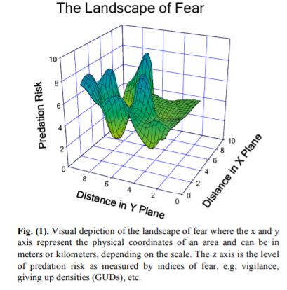
But what about the prey? How do the prey structure themselves relative to their predators? This question is explored in depth in a paper titled “The Landscape of Fear: Ecological Implications of Being Afraid” (Laundre et al. 2010), which we discussed in our most recent lab meeting. When wolves were re-introduced in Yellowstone, the elk increased their vigilance and altered their grazing patterns. As a result, the plant community was altered to reflect this “landscape of fear” that the elk move through, where their distribution not only reflected opportunities for the elk to eat but also the risk of being eaten.
Translating the landscape of fear concept to the marine environment is tricky, but a fascinating exercise in ecological theory. We grappled with drawing parallels between the example system of wolves, elk, and vegetation and baleen whales, zooplankton, and phytoplankton. Relative to grazing mammals like elk, the cognitive abilities of zooplankton like krill, copepods, and mysid might pale in comparison. How could we possibly measure “fear” or “vigilance” in zooplankton? The swarming behavior of mysid and krill into dense patches is a defense mechanism—the strategy they have evolved to lessen the likelihood that any one of them will be eaten by a predator. I would posit that the diel vertical migration (DVM) of zooplankton is a manifestation of fear, at least on some level. DVM occurs over the course of each day, with plankton in pelagic ecosystems migrating vertically in the water column to avoid predators by hiding at depth during the daylight hours, and then swimming upward to feed on phytoplankton under the cover of darkness. I won’t speculate any further on the intelligence of zooplankton, but the need to survive predation has driven them to evolve this effective evolutionary strategy of hiding in the ocean’s twilight zone, swimming upward to feed only after dark so that they’re less likely to linger in spaces occupied by predators.
A swarm of mysid along the Oregon Coast. How does fear of predation by gray whales or rockfish drive the distribution of zooplankton in this shallow, nearshore system? Photo by Dawn Barlow.
A rock covered in purple urchin on the Oregon Coast. In the absence of their major predators (sea otters and sea stars), are urchins able to thrive in an environment with less fear of predation? Photo by Dawn Barlow.
A blue whale lunges on a dense aggregation of krill in New Zealand. In this image, you can actually see the krill “fleeing”, jumping out of the water in an attempt to escape the whale’s mouth. Drone piloted by Todd Chandler.
Laundre et al. (2010) present a visual representation of the landscape of fear (Fig. 1, reproduced below), where as an animal moves through space (represented as distance in meters or kilometers, for example), they also move through varying levels of predation risk. Environmental gradients (temperature, for example) tend to be much more stable across space in terrestrial ecosystems such as in the Yellowstone example from the paper. I wonder whether the same concept and visual depiction of a landscape of fear could be translated as risk across various environmental gradients, rather than geographic distances? In this proposed illustration, a landscape of fear would vary based on gradients of environmental conditions rather than geographic space. Such a shift in spatial reference —from geographic to environmental space—might make the model more applicable in the dynamic ocean ecosystems that we study.
What about cases when the predators we study become prey? One example we discussed was gray whales migrating from breeding lagoons in Mexico to feeding grounds in the Bering Sea. Mother-calf pairs hug the coastline tightly, by no means taking the most direct route between locations and adding considerable travel distance to their migration. The leading hypothesis is that mother gray whales take the coastal route to minimize the risk that their calves will fall prey to killer whale attacks. Are there other cases where the predators we study operate in a seascape of fear that we do not yet understand? Likely so, and the predators’ own seascape of fear may account for cases when we cannot explain predator distribution simply by their prey and their environment. To take this a step further, it might be beneficial not only to think of predation risk as only the potential to be eaten, but expand our definition to include human disturbance. While humans may not directly prey on marine predators, the disturbance from human activity in the ocean likely creates a layer of fear which animals must navigate, even in the absence of actual predation.
Our lively lab meeting discussion prompted me to look into
how the landscape of fear model has been applied to the highly dynamic and
intricate marine environment. In a study examining predator-prey dynamics of
three species of marine mammals—bottlenose dolphins, harbor seals, and
dugongs—Wirsing et al. (2007) found that in all three cases, the study species
spent less time in more desirable prey patches or decreased riskier behavior in
the presence of predators. Most studies in marine ecology are observational, as
we rarely have the opportunity to manipulate our study system for experimental
design and hypothesis testing. However, a study of coral reefs in the Florida
Keys conducted by Catano et al. (2015) used fabricated predators—decoys of
black grouper, a predatory fish—to investigate the influence of fear of
predation on the reef system. What they found was that herbivorous fish
consumed significantly less and fed at a much faster rate in the presence of this
decoy predator. The grouper, even in decoy form, created a “reefscape of fear”,
altering patterns in herbivory with potential ramifications for the entire ecosystem.
My takeaway from our discussion and my musings in this
week’s blog post is that predator and prey distribution and behavior is highly
interconnected. While predators distribute themselves to maximize their ability
to find a meal, their prey respond accordingly by balancing finding a meal of
their own with minimizing the risk that they will be eaten. Ecology is the
study of an ecosystem, which means the questions we ask are complicated and
hierarchical, and must be considered from multiple angles, accounting for
biological, environmental, and behavioral elements to name a few. These
challenges of studying ecosystems are simultaneously what make ecology
fascinating, and exciting.
References:
Laundré, J. W., Hernández, L., & Ripple, W. J. (2010).
The landscape of fear: ecological implications of being afraid. Open
Ecology Journal, 3, 1-7.
Catano, L. B., Rojas, M. C., Malossi, R. J., Peters, J. R.,
Heithaus, M. R., Fourqurean, J. W., & Burkepile, D. E. (2016). Reefscapes
of fear: predation risk and reef hetero‐geneity interact to shape herbivore
foraging behaviour. Journal of Animal Ecology, 85(1),
146-156.
Wirsing, A. J., Heithaus, M. R., Frid, A., & Dill, L. M.
(2008). Seascapes of fear: evaluating sublethal predator effects experienced
and generated by marine mammals. Marine Mammal Science, 24(1),
1-15.
By: Alexa Kownacki, Ph.D. Student, OSU Department of Fisheries and Wildlife, Geospatial Ecology of Marine Megafauna Lab
Data analysis is often about parsing down data into manageable subsets. My project, which spans 34 years and six study sites along the California coast, requires significant data wrangling before full analysis. As part of a data analysis trial, I first refined my dataset to only the San Diego survey location. I chose this dataset for its standardization and large sample size; the bulk of my sightings, over 4,000 of the 6,136, are from the San Diego survey site where the transect methods were highly standardized. In the next step, I selected explanatory variable datasets that covered the sighting data at similar spatial and temporal resolutions. This small endeavor in analyzing my data was the first big leap into understanding what questions are feasible in terms of variable selection and analysis methods. I developed four major hypotheses for this San Diego site.
The study species: common bottlenose dolphin (Tursiops truncatus) seen along the California coastline in 2015. Image source: Alexa Kownacki.
Hypotheses:
H1: I predict that bottlenose dolphin sightings along the San Diego transect throughout the years 1981-2015 exhibit clustered distribution patterns as a result of the patchy distributions of both the species’ preferred habitats, as well as the social nature of bottlenose dolphins.
H2: I predict there would be higher densities of bottlenose dolphin at higher latitudes spanning 1981-2015 due to prey distributions shifting northward and less human activities in the northerly sections of the transect.
H3: I predict that during warm (positive) El Niño Southern Oscillation (ENSO) months, the dolphin sightings in San Diego would be distributed more northerly, predominantly with prey aggregations historically shifting northward into cooler waters, due to (secondarily) increasing sea surface temperatures.
H4: I predict that along the San Diego coastline, bottlenose dolphin sightings are clustered within two kilometers of the six major lagoons, with no specific preference for any lagoon, because the murky, nutrient-rich waters in the estuarine environments are ideal for prey protection and known for their higher densities of schooling fishes.
Data Description:
The common bottlenose dolphin (Tursiops truncatus) sighting data spans 1981-2015 with a few gap years. Sightings cover all months, but not in all years sampled. The same transect in San Diego was surveyed in a small, rigid-hulled inflatable boat with approximately a two-kilometer observation area (one kilometer surveyed 90 degrees to starboard and port of the bow).
I wanted to see if there were changes in dolphin distribution by latitude and, if so, whether those changes had a relationship to ENSO cycles and/or distances to lagoons. For ENSO data, I used the NOAA database that provides positive, neutral, and negative indices (1, 0, and -1, respectively) by each month of each year. I matched these ENSO data to my month-date information of dolphin sighting data. Distance from each lagoon was calculated for each sighting.
Figure 1. Map representing the San Diego transect, represented with a light blue line inside of a one-kilometer buffered “sighting zone” in pale yellow. The dark pink shapes are dolphin sightings from 1981-2015, although some are stacked on each other and cannot be differentiated. The lagoons, ranging in size, are color-coded. The transect line runs from the breakwaters of Mission Bay, CA to Oceanside Harbor, CA.
Results:
H1:True, dolphins are clustered and do not have a uniform distribution across this area. Spatial analysis indicated a less than a 1% likelihood that this clustered pattern could be the result of random chance (Fig. 1, z-score = -127.16, p-value < 0.0001). It is well-known that schooling fishes have a patchy distribution, which could influence the clustered distribution of their dolphin predators. In addition, bottlenose dolphins are highly social and although pods change in composition of individuals, the dolphins do usually transit, feed, and socialize in small groups.
Figure 2. Summary from the Average Nearest Neighbor calculation in ArcMap 10.6 displaying that bottlenose dolphin sightings in San Diego are highly clustered. When the z-score, which corresponds to different colors on the graphic above, is strongly negative (< -2.58), in this case dark blue, it indicates clustering. Because the p-value is very small, in this case, much less than 0.01, these results of clustering are strongly significant.
H2:False, dolphins do not occur at higher densities in the higher latitudes of the San Diego study site. The sightings are more clumped towards the lower latitudes overall (p < 2e-16), possibly due to habitat preference. The sightings are closer to beaches with higher human densities and human-related activities near Mission Bay, CA. It should be noted, that just north of the San Diego transect is the Camp Pendleton Marine Base, which conducts frequent military exercises and could deter animals.
Figure 3. Histogram comparing the latitudes with the frequency of dolphin sightings in San Diego, CA. The x-axis represents the latitudinal difference from the most northern part of the transect to each dolphin sighting. Therefore, a small difference would translate to a sighting being in the northern transect areas whereas large differences would translate to sightings being more southerly. This could be read from left to right as most northern to most southern. The y-axis represents the frequency of which those differences are seen, that is, the number of sightings with that amount of latitudinal difference, or essentially location on the transect line. Therefore, you can see there is a peak in the number of sightings towards the southern part of the transect line.
H3: False, during warm (positive) El Niño Southern Oscillation (ENSO) months, the dolphin sightings in San Diego were more southerly. In colder (negative) ENSO months, the dolphins were more northerly. The differences between sighting latitude and ENSO index was significant (p<0.005). Post-hoc analysis indicates that the north-south distribution of dolphin sightings was different during each ENSO state.
Figure 4. Boxplot visualizing distributions of dolphin sightings latitudinal differences and ENSO index, with -1,0, and 1 representing cold, neutral, and warm years, respectively.
H4:True, dolphins are clustered around particular lagoons. Figure 5 illustrates how dolphin sightings nearest to Lagoon 6 (the San Dieguito Lagoon) are always within 0.03 decimal degrees. Because of how these data are formatted, decimal degrees is the easiest way to measure change in distance (in this case, the difference in latitude). In comparison, dolphins at Lagoon 5 (Los Penasquitos Lagoon) are distributed across distances, with the most sightings further from the lagoon.
Figure 5. Bar plot displaying the different distances from dolphin sighting location to the nearest lagoon in San Diego in decimal degrees. Note: Lagoon 4 is south of the study site and therefore was never the nearest lagoon.
I found a significant difference between distance to nearest lagoon in different ENSO index categories (p < 2.55e-9): there is a significant difference in distance to nearest lagoon between neutral and negative values and positive and neutral years. Therefore, I hypothesize that in neutral ENSO months compared to positive and negative ENSO months, prey distributions are changing. This is one possible hypothesis for the significant difference in lagoon preference based on the monthly ENSO index. Using a violin plot (Fig. 6), it appears that Lagoon 5, Los Penasquitos Lagoon, has the widest variation of sighting distances in all ENSO index conditions. In neutral years, Lagoon 0, the Buena Vista Lagoon has multiple sightings, when in positive and negative years it had either no sightings or a single sighting. The Buena Vista Lagoon is the most northerly lagoon, which may indicate that in neutral ENSO months, dolphin pods are more northerly in their distribution.
Figure 6. Violin plot illustrating the distance from lagoons of dolphin sightings under different ENSO conditions. There are three major groups based on ENSO index: “-1” representing cold years, “0” representing neutral years, and “1” representing warm years. On the x-axis are lagoon IDs and on the y-axis is the distance to the nearest lagoon in decimal degrees. The wider the shapes, the more sightings, therefore Lagoon 6 has many sightings within a very small distance compared to Lagoon 5 where sightings are widely dispersed at greater distances.
Bottlenose dolphins foraging in a small group along the California coast in 2015. Image source: Alexa Kownacki.
Takeaways to science and management:
Bottlenose dolphins have a clustered distribution which seems to be related to ENSO monthly indices, and likely, their social structures. From these data, neutral ENSO months appear to have something different happening compared to positive and negative months, that is impacting the sighting distributions of bottlenose dolphins off the San Diego coastline. More research needs to be conducted to determine what is different about neutral months and how this may impact this dolphin population. On a finer scale, the six lagoons in San Diego appear to have a spatial relationship with dolphin sightings. These lagoons may provide critical habitat for bottlenose dolphins and/or for their preferred prey either by protecting the animals or by providing nutrients. Different lagoons may have different spans of impact, that is, some lagoons may have wider outflows that create larger nutrient plumes.
Other than the Marine Mammal Protection Act and small protected zones, there are no safeguards in place for these dolphins, whose population hovers around 500 individuals. Therefore, specific coastal areas surrounding lagoons that are more vulnerable to habitat loss, habitat degradation, and/or are more frequented by dolphins, may want greater protection added at a local, state, or federal level. For example, the Batiquitos and San Dieguito Lagoons already contain some Marine Conservation Areas with No-Take Zones within their reach. The city of San Diego and the state of California need better ways to assess the coastlines in their jurisdictions and how protecting the marine, estuarine, and terrestrial environments near and encompassing the coastlines impacts the greater ecosystem.
This dive into my data was an excellent lesson in spatial scaling with regards to parsing down my data to a single study site and in matching my existing data sets to other data that could help answer my hypotheses. Originally, I underestimated the robustness of my data. At first, I hesitated when considering reducing the dolphin sighting data to only include San Diego because I was concerned that I would not be able to do the statistical analyses. However, these concerns were unfounded. My results are strongly significant and provide great insight into my questions about my data. Now, I can further apply these preliminary results and explore both finer and broader scale resolutions, such as using the more precise ENSO index values and finding ways to compare offshore bottlenose dolphin sighting distributions.