The ecologist and the economist: Exploring parallels between disciplines

By Dawn Barlow1 and Johanna Rayl2

1PhD Candidate, Oregon State University Department of Fisheries and Wildlife, Geospatial Ecology of Marine Megafauna Lab

2PhD Student, Northwestern University Department of Economics

The Greek word “oikos” refers to the household and serves as the root of the words ecology and economics. Although perhaps surprising, the common origin reflects a shared set of basic questions and some shared theoretical foundations related to the study of how lifeforms on earth use scarce resources and find equilibrium in their respective “households”. Early ecological and economic theoretical texts drew inspiration from one another in many instances. Paul Samuelson, fondly referred to as “the father of modern economics,” observed in his defining work Foundations of Economic Analysis that the moving equilibrium in a market with supply and demand is “essentially identical with the moving equilibrium of a biological or chemical system undergoing slow change.” Likewise, early theoretical ecologists recognized the strength of drawing on theories previously established in economics (Real et al. 1991). Similar broad questions are central to researchers in both fields; in a large and dynamic system (termed “macro” in economics) scale, ecologists and economists alike work to understand where competitive forces find equilibrium, and an in individual (or micro) scale, they ask how individuals make behavior choices to maximize success given constraints like time, energy, wealth, or physical resources.

The central model economists have in mind when trying to understand human choices involves “constrained optimization”: what decision will maximize a person, family, firm, or other agent’s objectives given their limitations? For example, someone that enjoys relaxing but also seeks a livable income must choose how much time to devote to working versus relaxing, given the constraint of having just 24 hours in the day, and given the wage they receive from working. An economist studying this decision may want to learn about how changes in the wage will affect that person’s choice of working hours, or how much they dislike working relative to relaxing. Along similar lines, early ecologists theorized that organisms could be selected for one of two optimization strategies: minimizing the time spent acquiring a given amount of energy (i.e., calories from food), or maximizing total energy acquisition per unit of time (Real et al. 1991). Foundational work in the field of economics clarified numerous technical details about formulating and solving such optimization problems. Returning to the example of the leisure time decision, economic theory asks: does it matter if we model this decision as maximizing income given wages and limited time, or as minimizing hours spent working given a desired lifetime income?; can we formulate a “utility function” that  describes how well-off someone is with a given income and amount of leisure?; can we solve for the optimal amount of leisure with pen and paper? The toolkit arising from this work serves as a jumping off point for all contemporary economic research, and the kinds of choices understood under this framework is vast, from, where should a child attend school?; to, how should a government allocate its budget across public resources?

Early work in ecology drew from foundational concepts in economics, following the realization that the strategies by which organisms exploit resources most efficiently also involve optimization. This parallel was articulated by MacArthur and Pianka in their foundational 1966 paper Optimal Use of a Patchy Environment, in which they state: “In this paper we undertake to determine in which patches a species would feed and which items would form its diet if the species acted in the most economical fashion. Hopefully, natural selection will often have achieved such optimal allocation of time and energy expenditures.” Subsequently, this idea was refined into what is known in ecology as the marginal value theorem, which states that an animal should remain in a prey patch until the rate of energy gain drops below the expected energy gain in all remaining available patches (Charnov 1976). In other words, if it is more profitable to switch prey patches than to stay, an animal should move on. These optimization models therefore allow ecologists to pose specific evolutionary and behavioral hypotheses, such as examining energy acquisition over time to understand selective forces on foraging behavior.

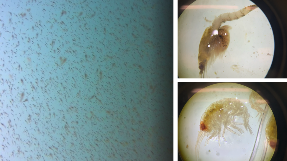
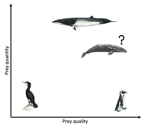
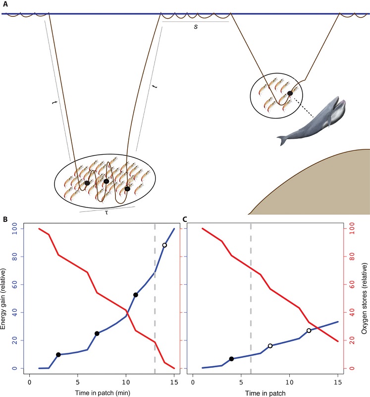
As the largest animals on the planet, blue whales have massive prey requirements to meet energy demands. However, they must balance their need to feed with costs such as oxygen consumption during breath-holding, the travel time it takes to reach prey patches at depth, the physiological constraints of diving, and the necessary recuperation time at the surface. It has been demonstrated that blue whales forage selectively to optimize this energetic budget. Therefore, blue whales should only feed on krill aggregations when the energetic gain outweighs the cost (Fig. 1), and this pattern has been empirically demonstrated for blue whale populations in the Gulf of St. Lawrence, Canada (Doniol-Valcroze et al. 2011), in the California Current, (Hazen et al. 2015) and in New Zealand (Torres et al. 2020).

Figure 1. Figure reprinted from Hazen et al. 2015, illustrating how a blue whale should theoretically optimize foraging success in two scenarios. Energy gained from feeding is shown by the blue lines, whereas the cost of foraging in terms of declining oxygen stores during a dive is illustrated by the red lines. On the left (panel B), the whale maximizes its energy gain by increasing the number of feeding lunges (shown by black circles) at the expense of declining oxygen stores when prey density is high. On the right (panel C), the whale minimizes oxygen use by reducing the number of feeding lunges when prey density is low.

The notion of the marginal value theorem is likewise at work in countless economic settings. Economic theory predicts that a farmer cultivating two crops would allocate resources into each crop such that the returns to adding more resources into each crop are the same. If not, she should move resources from the less productive crop to the one where marginal gains are larger. A fisherman, according to this notion, continues to fish longer into the season until the marginal value of one additional day at sea equals the marginal cost of their time, effort, and expenses. These predictions are intuitive by the same logic as the blue whale choosing where to forage, and derive from the mathematics of constrained and unconstrained optimization. Reassuringly, empirical work finds evidence of such profit-maximizing behavior in many settings. In a recent working paper, Burlig, Preonas, and Woerman explore how farmers’ water use in California responds to changes in the price of electricity, which effectively makes groundwater irrigation more expensive due to electric pumping. They find that farmers are very responsive to these changes in marginal cost. Farmers achieve this reduction in water use predominantly by switching to less water-intensive crops and fallowing their land (Burlig, Preonas, and Woerman 2020).

Undoubtedly there are fundamental differences between an ecosystem with interacting biotic and abiotic components and the human-economic environment with its many social and political structures. But for certain types of questions, the parallels across the shared optimization problems are striking. The foundational theories discussed here have paved the way for subsequent advances in both disciplines. For example, the field of behavioral ecology explores how competition and cooperation between and within species affects fitness of populations. Reflecting on early seminal work lends some perspective on how an area of research has evolved. Likewise, exploring parallels between disciplines sheds light on common threads, in turn revealing insights into each discipline individually.

References:

Burlig, Fiona, Louis Preonas, and Matt Woerman (2020). Groundwater, energy, and crop choice. Working Paper.

Charnov EL (1976) Optimal foraging: The marginal value theorem. Theoretical Population Biology 9:129–136.

Doniol-Valcroze T, Lesage V, Giard J, Michaud R (2011) Optimal foraging theory predicts diving and feeding strategies of the largest marine predator. Behavioral Ecology 22:880–888.

Hazen EL, Friedlaender AS, Goldbogen JA (2015) Blue whales (Balaenoptera musculus) optimize foraging efficiency by balancing oxygen use and energy gain as a function of prey density. Science Advces 1:e1500469–e1500469.

MacArthur RH, Pianka ER (1966) On optimal use of a patchy environment. The American Naturalist 100:603–609.

Real LA, Levin SA, Brown JH (1991) Part 2: Theoretical advances: the role of theory in the rise of modern ecology. In: Foundations of ecology: classic papers with commentaries.

Samuelson, Paul (1947). Foundations of Economic Analysis. Harvard University Press.

Torres LG, Barlow DR, Chandler TE, Burnett JD (2020) Insight into the kinematics of blue whale surface foraging through drone observations and prey data. PeerJ 8:e8906.

Feasts of junk food or morsels of fine dining: is prey quality or quantity more important to marine predators?

By Lisa Hildebrand, MSc student, OSU Department of Fisheries & Wildlife, Marine Mammal Institute, Geospatial Ecology of Marine Megafauna Lab

Knowing what and how much prey a predator feeds on are key components to better understanding and conserving that predator. Prey abundance and availability are frequently predictors for marine predator reproductive success and population dynamics. It is the reason why the GEMM Lab makes a concerted effort to not only track our main taxa of interest (marine mammals) but to simultaneously measure their prey. However, over the last decade or two, there has been increased recognition that prey quality is also highly important in understanding a predator’s ecology (Spitz et al. 2012). Optimal foraging theory is a widely accepted framework that posits that predators should attempt to maximize energy gained and minimize energy spent during a foraging event (Charnov 1976, Krebs 1978, Pyke 1984). Thus, knowledge of how valuable a prey item is in terms of its energetic content is an important part of the equation when applying optimal foraging theory to a predator of interest.

Ideally, the prey species with the highest energetic value would also be the easiest, most ubiquitous and least energetically expensive prey item to capture and consume, such that a predator truly could expend very little energy to get very high energetic rewards. However, it rarely is this straightforward. The caloric content of several marine prey species has been shown to increase with increasing size (e.g. Benoit-Bird 2004; Fig. 1), both length and weight. Yet, increasing size often also means increased mobility and, as a result, ability to evade and escape predation. Furthermore, increasing size also inherently means decreasing abundances – there will always be billions more krill in the ocean than whales based solely on cost of reproduction. Therefore, just based on sheer numbers, there are fewer big prey items, which increases the time between, and decreases the likelihood of, a predator encountering big prey items. So, there are clear trade-offs here. It may take longer to locate and capture a high value prey item, which costs more energy to capture, but the payout could potentially be much bigger. However, if a predator gambles too much, then their net energy expenditure to obtain high value prey may be higher than the net energy gained. Instead, it may be worth pursuing smaller prey items with lower energetic values, where discovery and capture success are higher and more frequent. However, in this case, many, many more pursuits are likely needed, thus costing more energy to meet daily energetic demands. 

Figure 1. Increasing caloric content with increasing length (a) and wet weight (b). Figures and caption reproduced from Benoit-Bird 2004.

Is your head spinning as much as mine? Let me try and simplify this complex web of interactions with a tangible example. Bowen et al. (2002) investigated foraging of harbor seals in Nova Scotia to assess prey profitability of different species. By attaching camera systems to the backs of 39 adult male harbor seals, the authors identified sand lance and flounder to be the most targeted prey species. However, there were significant differences in pursuit/handling cost per prey type (kJ/min) with sand lance only requiring 14.8 ± 2.7, whereas flounder required significantly more at 30.3 ± 7.9. Therefore, based solely on energy required to capture prey, the sand lance would seem to be the better option. In fact, to a certain degree, this hypothesis is actually true when we compare the energetic content of the two prey types. Sand lance have a higher energetic value at lengths of 10 and 15 cm (53.6 and 95.8 kJ, respectively) compared to flounder (22.6 and 88.6 kJ, respectively). So, the net gain of a harbor seal foraging on a 15 cm sand lance (assuming that it only takes 1 minute to catch the fish – this is more for explanatory purposes as it likely takes much longer for a harbor seal to capture a fish) would be 81 kJ. This gain is larger than that of a 15 cm flounder (58.3 kJ). However, once we compare these fish at 20 and 25 cm lengths, the flounder actually becomes the more beneficial prey item at 232.6 and 492.3 kJ, respectively, over the sand lance (158.1 and 233.8 kJ). Now, assuming once again that it only takes 1 minute to catch the fish, the harbor seal enjoys a net energetic gain of a whopping 462 kJ when capturing a 25 cm flounder compared to 219 kJ for a sand lance of the same size – that makes the flounder more than twice as profitable!

The Bowen et al. study is an excellent demonstration of the importance of considering the quality of prey items when studying the ecology of marine predators. However, the authors did not assess the relative availability of sand lance and flounder. Ideally, foraging ecology studies aimed at understanding prey choice would try to address both important prey metrics – quality and quantity. This goal is the exact aim of my second Master’s thesis chapter where I am investigating whether prey quality (determined through community composition and caloric content) or prey quantity (measured as relative density) is more important in driving fine-scale gray whale foraging behavior in Port Orford, Oregon (Fig. 2). This question can be simplified by asking does it matter more what prey is in an area, or how much prey there is in an area? Or we can relate it back to the title of this post by asking whether individual gray whales would rather attend a cheap all-you-can-eat buffet or an expensive fine-dining restaurant. I am unfortunately not quite done with my analyses yet (but I’m getting closer!) and therefore am not ready to answer these questions. However, I have done extensive research on this topic and therefore am in a position to briefly mention a few other studies that have investigated these questions for other marine predators. 

Figure 2. A question of what or how much. Left image: example of the screenshots we take to estimate relative prey density in Port Orford. Right images: two examples of the main prey species we find (top: mysid shrimp Neomysis rayii with a full brood pouch; bottom: amphipod Polycheria osborni).

Ludynia et al. (2010) explored reasons why African penguin (Spehniscus demersus) numbers have declined in Namibia. They found that after the collapse of pelagic fish stocks in the 1970s (including the principal penguin prey item, sardine), African penguins switched to feeding on bearded goby, which are considered a low-energy prey species. Bearded goby are relatively abundant along Namibia’s southern coast and as such, limited prey availability is not the reason for declining African penguin numbers. Therefore, the authors concluded that the low quality of bearded goby (compared to sardine) appears to be the reason for declining population trends  of the penguins. This study demonstrates that African penguins do better when eating at a fine-dining restaurant, rather than loading up a whole plate of junk food. 

Grémillet et al. (2004) studied the foraging effort and number of successful prey captures per foraging trip (yield) of great cormorants (Phalacrocorax carbo) in Greenland in relation to prey abundance and quality within their foraging areas. The authors radio-tracked 11 great cormorants during a total of 163 foraging trips to estimate foraging effort and yield. The study found that contrary to the authors’ hypothesis, great cormorants foraged in areas of low prey abundance where the average caloric value was also relatively low. Therefore, in this example, it would seem that the predator of interest prioritizes neither high quality nor quantity when foraging.

Haug et al. (2002) investigated the variations in minke whale (Balaenoptera acutorostrata) diet and body condition in response to ecosystem changes in the Barents Sea. The main prey item of minke whales in the Barents Sea is immature herring. However, when recruitment failure and subsequent weak cohorts leads to reduced availability of immature herring, minke whales switched their diet to other prey items such as krill, capelin, and sometimes other gadoid fish species. The authors found a correlation between body condition of minke whales and immature herring abundances, such that minke whales displayed a poor body condition during low immature herring abundances. However, in the years of low immature herring abundance, abundances of krill and capelin were not low. Therefore, similar to the Ludynia et al. (2010) study, it seems that minke whales in the Barents Sea also do better in years when the prey type of highest caloric value is the most abundant. However, decreases in high quality prey has not led to population declines in minke whales in the Barents Sea, indicating that they likely take advantage of high quantities of low quality prey, unlike the African penguins.

Clearly, the answer as to whether marine predators prefer quality over quantity is not simple and constant. Rather, prey preference varies based on predator needs and ecology, falling anywhere on a broad spectrum from low to high prey quality and low to high prey quantity (Fig. 3). To a certain extent, it probably also is not solely predator choice that determines what they eat but many other factors, such as climate, disturbance, and health. As a result, these preferences and choices will likely be fluid, rather than fixed. While I anticipate that individual gray whales will be flexible foragers, I do hypothesize that when there is a prey patch of a higher energetic value in the area, whales will preferentially consume these patches over areas where there is less energetically rich prey, even if it is more abundant. 

Figure 3. A spectrum of prey quantity and quality. Giant cormorants forage on low prey quality & quantity (Grémillet et al. 2004). African penguin populations are declining despite high abundances of low quality prey, suggesting that high prey quality is important for their survival (Ludynia et al. 2010). Body condition of Barents Sea minke whales decreases when high quality prey is less abundant, however their populations have not declined, suggesting they instead exploit high abundances of low quality prey (Haug et al. 2002). What will the gray whales do?

Literature cited

Benoit-Bird, K. J. 2004. Prey caloric value and predator energy needs: foraging predictions for wild spinner dolphins. Marine Biology 145:435-444.

Bowen, W. D., D. Tuley, D. J. Boness, B. M. Bulheier, and G. J. Marshall. 2002. Prey-dependent foraging tactics and prey profitability in a marine mammal. Marine Ecology Progress Series 244:235-245.

Charnov, E. L. 1976. Optimal foraging, the marginal value theorem. Theoretical Population Biology 9(2):129-136.

Grémillet D., G. Kuntz, F. Delbart, M. Mellet, A. Kato, J-P. Robin, P-E. Chaillon, J-P. Gendner, S-H. Lorentsen, and Y. Le Maho. 2004. Linking the foraging performance of a marine predator to local prey abundance. Functional Ecology 18(6):793-801.

Haug, T., U. Lindstrøm, and K. T. Nilssen. 2002. Variations in minke whale (Balaenoptera acutorostrata) diet and body condition in response to ecosystem changes in the Barents Sea. Sarsia 87(6):409-422. 

Krebs, J. R. 1978. Optimal foraging: decision rules for predators. Behvaioral Ecology: An Evolutionary Approach, eds. Krebs, J. R., and N. B. Davies. Oxford: Blackwell. 

Ludynia, J., J-P. Roux, R. Jones, J. Kemper, and L. G. Underhill. 2010. Surviving off junk: low-energy prey dominates  the diet of African penguins Spheniscus demersus at Mercury Island, Namibia, between 1996 and 2009. African Journal of Marine Science 32(3):563-572.

Pyke, G. H. 1984. Optimal foraging theory: a critical review. Annual Reviews of Ecology and Systematics 15:523-575.

Spitz, J., A. W. Trites, V. Becquet, A. Brind’Amour, Y. Cherel, R. Galois, and V. Ridoux. 2012. Cost of living dictates what whales, dolphins and porpoises eat: the importance of prey quality on predator foraging strategies. PLoS ONE 7(11):e50096.

Young, J. K., B. A. Black, J. T. Clarke, S. V. Schonberg, and K. H. Dunton. 2017. Abundance, biomass and caloric content of Chukchi Sea bivalves and association with Pacific walrus (Odobenus rosmarus divergens) relative density and distribution in the northeastern Chukchi Sea. Deep-Sea Research Part II 144:125-141.